Cyclic Model Visualization

Visualize and animate a full cyclic model. This model is based on the jetcat rotor.

First, load the rotor. Notice how printing the rotor class reveals the details of the rotor result file.

# sphinx_gallery_thumbnail_number = 2
from ansys.mapdl.reader import examples

rotor = examples.download_sector_modal()
print(rotor)

PyMAPDL Result
Units       : User Defined
Version     : 15.0
Cyclic      : True
Result Sets : 48
Nodes       : 460
Elements    : 210


Available Results:
EMS : Miscellaneous summable items (normally includes face pressures)
ENF : Nodal forces
ENS : Nodal stresses
ENG : Element energies and volume
EEL : Nodal elastic strains
ETH : Nodal thermal strains (includes swelling strains)
EUL : Element euler angles
EPT : Nodal temperatures
NSL : Nodal displacements
RF  : Nodal reaction forces

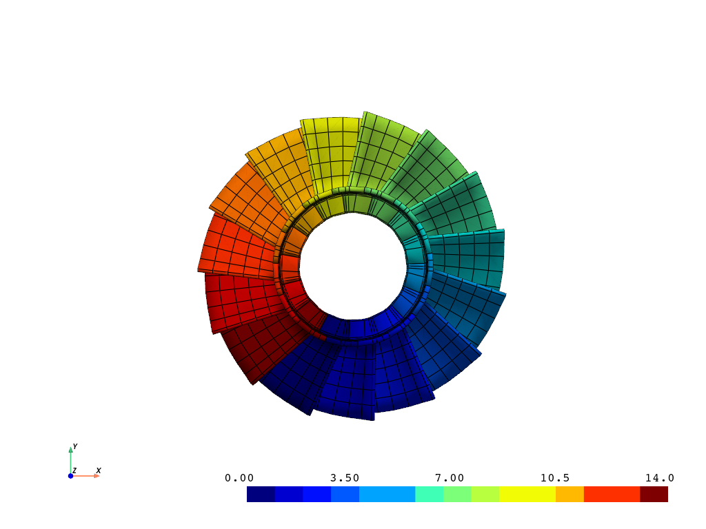
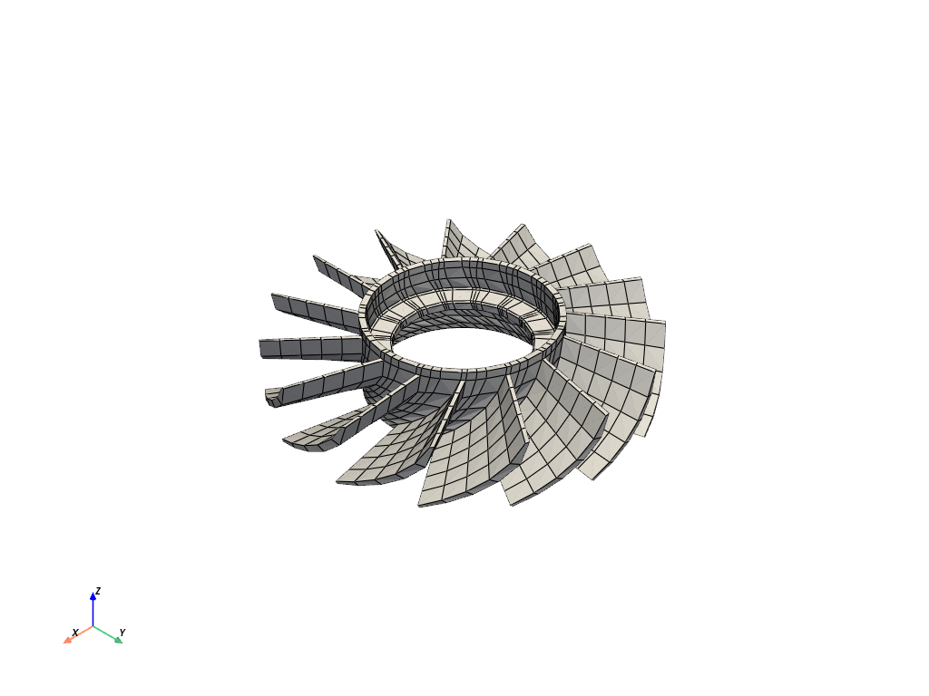
Plot the rotor and rotor sectors

Note that additional keyword arguments can be passed to the plotting functions of pymapdl-reader. See help(pyvista.plot for the documentation on all the keyword arguments.

rotor.plot_sectors(cpos="xy", smooth_shading=True)
rotor.plot()

• 
• 

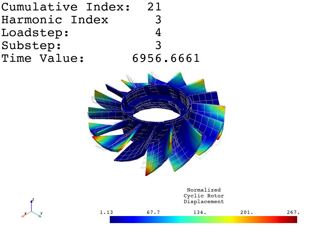
Plot nodal displacement for result 21.

Note that pymapdl-reader uses 0 based cumulative indexing. You could also use the (load step, sub step) (4, 3).

rotor.plot_nodal_displacement(
    20, show_displacement=True, displacement_factor=0.001, overlay_wireframe=True
)  # same as (2, 4)

Animate Mode 21

Disable movie_filename and increase n_frames for a smoother plot

rotor.animate_nodal_solution(
    20,
    loop=False,
    movie_filename="rotor_mode.gif",
    background="w",
    displacement_factor=0.001,
    add_text=False,
    n_frames=30,
)

[(5.52155060432921, 5.5214282518334326, 5.110814907184016),
 (3.164628201712816e-07, -0.00012203603295768417, -0.41073538068237303),
 (0.0, 0.0, 1.0)]