Reading MAPDL Result Files

The ansys-mapdl-reader module supports the following result types from MAPDL:

• ".rfl"

• ".rmg"

• ".rst"

• ".rth"

The MAPDL result file is a FORTRAN formatted binary file containing the results written from a MAPDL analysis. The results, at a minimum, contain the geometry of the model analyzed along with the nodal and element results. Depending on the analysis, these results could be anything from modal displacements to nodal temperatures. This includes (and is not limited to):

• Nodal DOF results from a static analysis or modal analysis.

• Nodal DOF results from a cyclic static or modal analysis.

• Nodal averaged component stresses (i.e. x, y, z, xy, xz, yz)

• Nodal principal stresses (i.e. S1, S2, S3, SEQV, SINT)

• Nodal elastic, plastic, and thermal stress

• Nodal time history

• Nodal boundary conditions and force

• Nodal temperatures

• Nodal thermal strain

• Various element results (see element_solution_data)

This module will likely change or depreciated in the future, and you are encouraged to checkout the new Data Processing Framework (DPF) modules at DPF-Core and DPF-Post as they provide a modern interface to ANSYS result files using a client/server interface using the same software used within ANSYS Workbench, but via a Python client.

Loading the Result File

As the MAPDL result files are binary files, the entire file does not need to be loaded into memory in order to retrieve results. This module accesses the results through a python object result which you can initialize with:

from ansys.mapdl import reader as pymapdl_reader
result = pymapdl_reader.read_binary('file.rst')

Upon initialization the Result object contains several properties to include the time values from the analysis, node numbering, element numbering, etc.

The ansys-mapdl-reader module can determine the correct result type by reading the header of the file, which means that if it is an MAPDL binary file, ansys-mapdl-reader can probably read it (at least to some degree. For example, a thermal result file can be read with

rth = pymapdl_reader.read_binary('file.rth')

Result Properties

The properties of the Result can be quickly shown by printing the result file with:

>>> result = pymapdl_reader.read_binary('file.rst')
>>> print(result)
PyMAPDL Result file object
Units       : User Defined
Version     : 20.1
Cyclic      : False
Result Sets : 1
Nodes       : 321
Elements    : 40


Available Results:
EMS : Miscellaneous summable items (normally includes face pressures)
ENF : Nodal forces
ENS : Nodal stresses
ENG : Element energies and volume
EEL : Nodal elastic strains
ETH : Nodal thermal strains (includes swelling strains)
EUL : Element euler angles
EPT : Nodal temperatures
NSL : Nodal displacements
RF  : Nodal reaction forces

To obtain the time or frequency values of an analysis use:

>>> result.time_values
array([1.])

Individual results can be obtained with one of the many methods available to the result object. For example, the nodal displacement for the first result can be accessed with:

>>> nnum, disp = rst.nodal_displacement(0)
>>> nnum
array([  1,   2,   3, ..., 318, 319, 320, 321], dtype=int32)

>>> disp
array([[-2.03146520e-09, -3.92491045e-03,  5.00047448e-05],
       [ 1.44630651e-09,  1.17747356e-02, -1.49992672e-04],
       [ 0.00000000e+00,  0.00000000e+00,  0.00000000e+00],
       ...
       [-7.14982194e-03,  3.12495002e-03,  5.74992265e-04],
       [-7.04982329e-03,  2.44996706e-03,  5.74992939e-04],
       [-6.94982520e-03,  1.77498362e-03,  5.74992891e-04]])

The sorted node and element numbering of a result can be obtained with:

>>> rst.geometry.nnum
array([  1,   2,   3, ..., 318, 319, 320, 321], dtype=int32)

>>> result.geometry.enum
array([ 1,  3,  2,  4,  5,  7,  6,  8,  9, 11, 10, 12, 13, 15, 14, 16, 17,
       19, 18, 20, 21, 23, 22, 24, 25, 27, 26, 28, 29, 31, 30, 32, 33, 35,
       34, 36, 37, 39, 38, 40], dtype=int32)

Mesh

The mesh of the result can be found by querying the mesh property of a result, which returns a ansys.mapdl.reader.mesh.Mesh class.

>>> from ansys.mapdl import reader as pymapdl_reader
>>> from ansys.mapdl.reader import examples
>>> rst = pymapdl_reader.read_binary(examples.rstfile)
>>> print(rst.mesh)

ANSYS Mesh
  Number of Nodes:              321
  Number of Elements:           40
  Number of Element Types:      1
  Number of Node Components:    0
  Number of Element Components: 0

Which contains the following attributes:

class ansys.mapdl.reader.mesh.Mesh(nnum=None, nodes=None, elem=None, elem_off=None, ekey=None, node_comps={}, elem_comps={}, rdat=[], rnum=[], keyopt={})

Common class between Archive, and result mesh

property ekey

Element type key

Array containing element type numbers in the first column and the element types (like SURF154) in the second column.

Examples

>>> from ansys.mapdl import reader as pymapdl_reader
>>> from ansys.mapdl.reader import examples
>>> archive = pymapdl_reader.Archive(examples.hexarchivefile)
>>> archive.ekey
array([[  1,  45],
       [  2,  95],
       [  3,  92],
       [ 60, 154]], dtype=int32)

property elem

List of elements containing raw ansys information.

Each element contains 10 items plus the nodes belonging to the element. The first 10 items are:

• FIELD 0 : material reference number

• FIELD 1 : element type number

• FIELD 2 : real constant reference number

• FIELD 3 : section number

• FIELD 4 : element coordinate system

• FIELD 5 : death flag (0 - alive, 1 - dead)

• FIELD 6 : solid model reference

• FIELD 7 : coded shape key

• FIELD 8 : element number

• FIELD 9 : base element number (applicable to reinforcing elements only)

• FIELDS 10 - 30 : The nodes belonging to the element in ANSYS numbering.

Examples

>>> from ansys.mapdl import reader as pymapdl_reader
>>> from ansys.mapdl.reader import examples
>>> archive = pymapdl_reader.Archive(examples.hexarchivefile)
>>> archive.elem
[array([  1,   4,  19,  15,  63,  91, 286, 240,   3,  18,  17,
         16,  81, 276, 267, 258,  62,  90, 285, 239],
 array([  4,   2,   8,  19,  91,  44, 147, 286,   5,   7,  21,
         18, 109, 137, 313, 276,  90,  43, 146, 285],
 array([ 15,  19,  12,  10, 240, 286, 203, 175,  17,  20,  13,
         14, 267, 304, 221, 230, 239, 285, 202, 174],
...

property elem_real_constant

Real constant reference for each element.

Use the data within rlblock and rlblock_num to get the real constant datat for each element.

Examples

>>> from ansys.mapdl import reader as pymapdl_reader
>>> from ansys.mapdl.reader import examples
>>> archive = pymapdl_reader.Archive(examples.hexarchivefile)
>>> archive.elem_real_constant
array([ 1,  1,  1,  1,  1,  1,  1,  1,  1,  1,  1,  1,  1,  1,
        1,  1,  1,  1,  1,  1,  1,  1,  1,  1,  1,  1,  1,  1,
        1,  1,  1,  1,  1,  1,  1,  1,  1,  1,  1,  1,  1,  1,
        ...,
        1,  1,  1,  1,  1,  1,  1,  1,  1,  1, 61, 61, 61, 61,
       61, 61, 61, 61, 61, 61, 61, 61, 61, 61, 61, 61, 61, 61,
       61], dtype=int32)

property element_components

Element components for the archive.

Output is a dictionary of element components. Each entry is an array of MAPDL element numbers corresponding to the element component. The keys are element component names.

Examples

>>> from ansys.mapdl import reader as pymapdl_reader
>>> from ansys.mapdl.reader import examples
>>> archive = pymapdl_reader.Archive(examples.hexarchivefile)
>>> archive.element_components
{'ECOMP1 ': array([17, 18, 21, 22, 23, 24, 25, 26, 27, 28, 29,
                   30, 31, 32, 33, 34, 35, 36, 37, 38, 39, 40],
                   dtype=int32),
'ECOMP2 ': array([ 1, 2, 3, 4, 5, 6, 7, 8, 9, 10, 11, 12, 13,
                  14, 15, 16, 17, 18, 19, 20, 23, 24], dtype=int32)}

element_coord_system()

Element coordinate system number

Examples

>>> from ansys.mapdl import reader as pymapdl_reader
>>> from ansys.mapdl.reader import examples
>>> archive = pymapdl_reader.Archive(examples.hexarchivefile)
>>> archive.element_coord_system
array([0, 0, 0, 0, 0, 0, 0, 0, 0, 0, 0, 0, 0, 0, 0, 0, 0, 0, 0,
       0, 0, 0, 0, 0, 0, 0, 0, 0, 0, 0, 0, 0, 0, 0, 0, 0, 0, 0,
       0, 0], dtype=int32)

property enum

ANSYS element numbers.

Examples

>>> from ansys.mapdl import reader as pymapdl_reader
>>> from ansys.mapdl.reader import examples
>>> archive = pymapdl_reader.Archive(examples.hexarchivefile)
>>> archive.enum
array([    1,     2,     3, ...,  9998,  9999, 10000])

property et_id

Element type id (ET) for each element.

property etype

Element type of each element.

This is the ansys element type for each element.

Examples

>>> from ansys.mapdl import reader as pymapdl_reader
>>> from ansys.mapdl.reader import examples
>>> archive = pymapdl_reader.Archive(examples.hexarchivefile)
>>> archive.etype
array([ 45,  45,  45,  45,  45,  45,  45,  45,  45,  45,  45,
        45,  45,  45,  45,  45,  45,  45,  45,  92,  92,  92,
        92,  92,  92,  92,  92,  92,  92,  92,  92,  92,  92,
        ...,
        92,  92,  92,  92,  92, 154, 154, 154, 154, 154, 154,
       154, 154, 154, 154, 154, 154, 154, 154, 154, 154, 154,
       154], dtype=int32)

Notes

Element types are listed below. Please see the APDL Element Reference for more details:

https://www.mm.bme.hu/~gyebro/files/vem/ansys_14_element_reference.pdf

property key_option

Additional key options for element types

Examples

>>> from ansys.mapdl import reader as pymapdl_reader
>>> from ansys.mapdl.reader import examples
>>> archive = pymapdl_reader.Archive(examples.hexarchivefile)
>>> archive.key_option
{1: [[1, 11]]}

property material_type

Material type index of each element in the archive.

Examples

>>> from ansys.mapdl import reader as pymapdl_reader
>>> from ansys.mapdl.reader import examples
>>> archive = pymapdl_reader.Archive(examples.hexarchivefile)
>>> archive.material_type
array([1, 1, 1, 1, 1, 1, 1, 1, 1, 1, 1, 1, 1, 1, 1, 1, 1, 1,
       1, 1, 1, 1, 1, 1, 1, 1, 1, 1, 1, 1, 1, 1, 1, 1, 1, 1,
       1, 1, 1, 1], dtype=int32)

property n_elem

Number of nodes

property n_node

Number of nodes

property nnum

Array of node numbers.

Examples

>>> from ansys.mapdl import reader as pymapdl_reader
>>> from ansys.mapdl.reader import examples
>>> archive = pymapdl_reader.Archive(examples.hexarchivefile)
>>> archive.nnum
array([    1,     2,     3, ..., 19998, 19999, 20000])

property node_angles

Node angles from the archive file.

Examples

>>> from ansys.mapdl import reader as pymapdl_reader
>>> from ansys.mapdl.reader import examples
>>> archive = pymapdl_reader.Archive(examples.hexarchivefile)
>>> archive.nodes
[[0.   0.   0.  ]
 [0.   0.   0.  ]
 [0.   0.   0.  ]
 ...,
 [0.   0.   0.  ]
 [0.   0.   0.  ]
 [0.   0.   0.  ]]

property node_components

Node components for the archive.

Output is a dictionary of node components. Each entry is an array of MAPDL node numbers corresponding to the node component. The keys are node component names.

Examples

>>> from ansys.mapdl import reader as pymapdl_reader
>>> from ansys.mapdl.reader import examples
>>> archive = pymapdl_reader.Archive(examples.hexarchivefile)
>>> archive.node_components
{'NCOMP2  ': array([  1,   2,   3,   4,   5,   6,   7,   8,
                     14, 15, 16, 17, 18, 19, 20, 21, 43, 44,
                     62, 63, 64, 81, 82, 90, 91, 92, 93, 94,
                     118, 119, 120, 121, 122, 123, 124, 125,
                     126, 137, 147, 148, 149, 150, 151, 152,
                     153, 165, 166, 167, 193, 194, 195, 202,
                     203, 204, 205, 206, 207, 221, 240, 258,
                     267, 268, 276, 277, 278, 285, 286, 287,
                     304, 305, 306, 313, 314, 315, 316
                     ], dtype=int32),
...,
}

property nodes

Array of nodes.

Examples

>>> from ansys.mapdl import reader as pymapdl_reader
>>> from ansys.mapdl.reader import examples
>>> archive = pymapdl_reader.Archive(examples.hexarchivefile)
>>> archive.nodes
[[0.   0.   0.  ]
 [1.   0.   0.  ]
 [0.25 0.   0.  ]
 ...,
 [0.75 0.5  3.5 ]
 [0.75 0.5  4.  ]
 [0.75 0.5  4.5 ]]

property rlblock

Real constant data from the RLBLOCK.

Examples

>>> from ansys.mapdl import reader as pymapdl_reader
>>> from ansys.mapdl.reader import examples
>>> archive = pymapdl_reader.Archive(examples.hexarchivefile)
>>> archive.rlblock
[[0.   , 0.   , 0.   , 0.   , 0.   , 0.   , 0.02 ],
 [0.   , 0.   , 0.   , 0.   , 0.   , 0.   , 0.01 ],
 [0.   , 0.   , 0.   , 0.   , 0.   , 0.   , 0.005],
 [0.   , 0.   , 0.   , 0.   , 0.   , 0.   , 0.005]]

property rlblock_num

Indices from the real constant data

Examples

>>> from ansys.mapdl import reader as pymapdl_reader
>>> from ansys.mapdl.reader import examples
>>> archive = pymapdl_reader.Archive(examples.hexarchivefile)
>>> archive.rnum
array([60, 61, 62, 63])

save(filename, binary=True, force_linear=False, allowable_types=[], null_unallowed=False)

Save the geometry as a vtk file

Parameters:

• filename (str, pathlib.Path) – Filename of output file. Writer type is inferred from the extension of the filename.

• binary (bool, optional) – If True, write as binary, else ASCII.

• force_linear (bool, optional) – This parser creates quadratic elements if available. Set this to True to always create linear elements. Defaults to False.

• allowable_types (list, optional) –

  Allowable element types. Defaults to all valid element types in ansys.mapdl.reader.elements.valid_types

  See help(ansys.mapdl.reader.elements) for available element types.

• null_unallowed (bool, optional) – Elements types not matching element types will be stored as empty (null) elements. Useful for debug or tracking element numbers. Default False.

Examples

>>> geom.save('mesh.vtk')

Notes

Binary files write much faster than ASCII and have a smaller file size.

property section

Section number

Examples

>>> from ansys.mapdl import reader as pymapdl_reader
>>> from ansys.mapdl.reader import examples
>>> archive = pymapdl_reader.Archive(examples.hexarchivefile)
>>> archive.section
array([1, 1, 1, 1, 1, 1, 1, 1, 1, 1, 1, 1, 1, 1, 1, 1, 1, 1, 1,
       1, 1, 1, 1, 1, 1, 1, 1, 1, 1, 1, 1, 1, 1, 1, 1, 1, 1, 1,
       1, 1], dtype=int32)

property tshape

Tshape of contact elements.

property tshape_key

Dict with the mapping between element type and element shape.

TShape is only applicable to contact elements.

Coordinate Systems

Non-default coordinate systems are always saved to a MAPDL result file. The coordinate system is zero indexed and individual coordinate systems can be accessed with:

>>> coord_idx = 12
>>> result.geometry['coord systems'][coord_idx]
{'transformation matrix': array([[ 0.0, -1.0,  0.0],
                                 [ 0.0,  0.0, -1.0],
                                 [ 1.0,  0.0,  0.0]]),
 'origin': array([0., 0., 0.]),
 'PAR1': 1.0,
 'PAR2': 1.0,
 'euler angles': array([ -0., -90.,  90.]),
 'theta singularity': 0.0,
 'phi singularity': 0.0,
 'type': 1,
 'reference num': 12}

A 4x4 transformation matrix can be constructed by concatenating the transformation matrix and the origin into one array. For example:

>>> cs = result.geometry['coord systems'][coord_idx]
>>> trans = cs['transformation matrix']
>>> origin = cs['origin']
>>> bottom = np.zeros(4)
>>> bottom[3] = 1
>>> tmat = np.hstack((trans, origin.reshape(-1 ,1)))
>>> tmat = np.vstack((tmat, bottom))

See parse_coordinate_system for more details regarding the contents of the coordinate systems stored in the result file.

Accessing Solution Results

You can obtain detailed information using solution_info for each result:

# return a dictionary of solution info for the first result
info = result.solution_info(0)

for key in info:
    print(key, info[key])

This yields:

timfrq 1.0
lfacto 1.0
lfactn 1.0
cptime 50.9189941460218
tref 0.0
tunif 0.0
tbulk 82.0
volbase 0.0
tstep 0.0
__unused 0.0
accel_x 0.0
accel_y 0.0
accel_z 0.0
omega_v_x 0.0
omega_v_y 0.0
omega_v_z 100
omega_a_x 0.0
omega_a_y 0.0
omega_a_z 0.0
omegacg_v_x 0.0
omegacg_v_y 0.0
omegacg_v_z 0.0
omegacg_a_x 0.0
omegacg_a_y 0.0
omegacg_a_z 0.0
cgcent 0.0
fatjack 0.0
dval1 0.0
pCnvVal 0.0

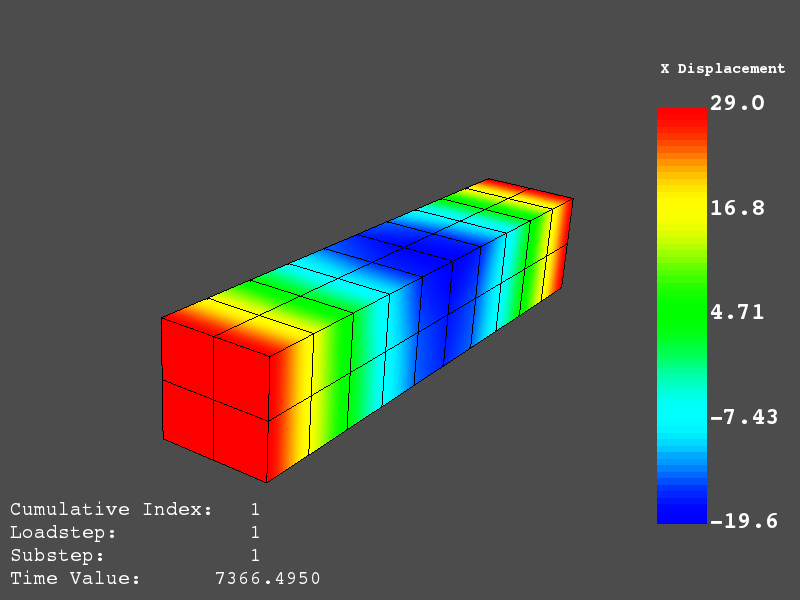
The DOF solution for an analysis for each node in the analysis can be obtained using the code block below. These results correspond to the node numbers in the result file. This array is sized by the number of nodes by the number of degrees of freedom.

# Return an array of results (nnod x dof)
nnum, disp = result.nodal_solution(0) # uses 0 based indexing

# where nnum is the node numbers corresponding to the displacement results

# The same results can be plotted using
result.plot_nodal_solution(0, 'x', label='Displacement') # x displacement

# normalized displacement can be plotted by excluding the direction string
result.plot_nodal_solution(0, label='Normalized')

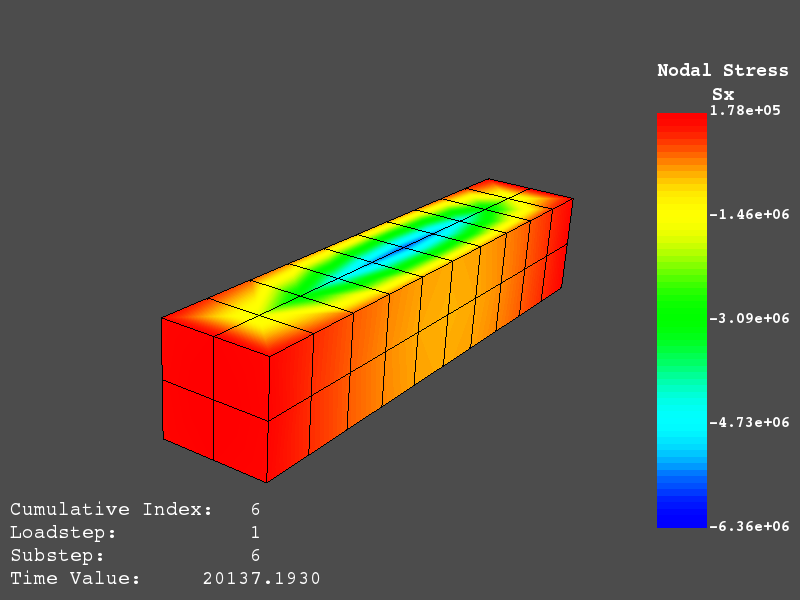
Stress can be obtained as well using the below code. The nodal stress is computed in the same manner as MAPDL by averaging the stress evaluated at that node for all attached elements.

# obtain the component node averaged stress for the first result
# organized with one [Sx, Sy Sz, Sxy, Syz, Sxz] entry for each node
nnum, stress = result.nodal_stress(0) # results in a np array (nnod x 6)

# Display node averaged stress in x direction for result 6
result.plot_nodal_stress(5, 'Sx')

# Compute principal nodal stresses and plot SEQV for result 1
nnum, pstress = result.principal_nodal_stress(0)
result.plot_principal_nodal_stress(0, 'SEQV')

Element stress can be obtained using the following segment of code. Ensure that the element results are expanded for a modal analysis within ANSYS with:

/SOLU
MXPAND, ALL, , , YES

This block of code shows how you can access the non-averaged stresses for the first result from a modal analysis.

from ansys.mapdl import reader as pymapdl_reader
result = pymapdl_reader.read_binary('file.rst')
estress, elem, enode = result.element_stress(0)

These stresses can be verified using MAPDL using:

>>> estress[0]
[[ 1.0236604e+04 -9.2875127e+03 -4.0922625e+04 -2.3697146e+03
  -1.9239732e+04  3.0364934e+03]
 [ 5.9612605e+04  2.6905924e+01 -3.6161423e+03  6.6281304e+03
   3.1407712e+02  2.3195926e+04]
 [ 3.8178301e+04  1.7534495e+03 -2.5156013e+02 -6.4841372e+03
  -5.0892783e+03  5.2503605e+00]
 [ 4.9787645e+04  8.7987168e+03 -2.1928742e+04 -7.3025332e+03
   1.1294199e+04  4.3000205e+03]]

>>> elem[0]
    32423

>>> enode[0]
    array([ 9012,  7614,  9009, 10920], dtype=int32)

Which are identical to the results from MAPDL:

POST1:
ESEL, S, ELEM, , 32423
PRESOL, S

***** POST1 ELEMENT NODAL STRESS LISTING *****

LOAD STEP=     1  SUBSTEP=     1
 FREQ=    47.852      LOAD CASE=   0

THE FOLLOWING X,Y,Z VALUES ARE IN GLOBAL COORDINATES

ELEMENT=   32423        SOLID187
  NODE    SX          SY          SZ          SXY         SYZ         SXZ
  9012   10237.     -9287.5     -40923.     -2369.7     -19240.      3036.5
  7614   59613.      26.906     -3616.1      6628.1      314.08      23196.
  9009   38178.      1753.4     -251.56     -6484.1     -5089.3      5.2504
 10920   49788.      8798.7     -21929.     -7302.5      11294.      4300.0

Loading a Results from a Modal Analysis Result File

This example reads in binary results from a modal analysis of a beam from ANSYS. This section of code does not rely on VTK and can be used with only numpy installed.

# Load the reader from pyansys
from ansys.mapdl import reader as pymapdl_reader
from ansys.mapdl.reader import examples

# Sample result file
rstfile = examples.rstfile

# Create result object by loading the result file
result = pymapdl_reader.read_binary(rstfile)

# Beam natural frequencies
freqs = result.time_values

>>> print(freqs)
[ 7366.49503969  7366.49503969 11504.89523664 17285.70459456
  17285.70459457 20137.19299035]

Get the 1st bending mode shape. Results are ordered based on the sorted node numbering. Note that results are zero indexed.

>>> nnum, disp = result.nodal_solution(0)
>>> print(disp)
[[ 2.89623914e+01 -2.82480489e+01 -3.09226692e-01]
 [ 2.89489249e+01 -2.82342416e+01  2.47536161e+01]
 [ 2.89177130e+01 -2.82745126e+01  6.05151053e+00]
 [ 2.88715048e+01 -2.82764960e+01  1.22913304e+01]
 [ 2.89221536e+01 -2.82479511e+01  1.84965333e+01]
 [ 2.89623914e+01 -2.82480489e+01  3.09226692e-01]
 ...

Accessing Element Solution Data

Individual element results for the entire solution can be accessed using the element_solution_data method. For example, to get the volume of each element:

import numpy as np
from ansys.mapdl import reader as pymapdl_reader

rst = pymapdl_reader.read_binary('./file.rst')
enum, edata = rst.element_solution_data(0, datatype='ENG')

# output as a list, but can be viewed as an array since
# the results for each element are the same size
edata = np.asarray(edata)
volume = edata[:, 0]

Animiating a Modal Solution

Solutions from a modal analysis can be animated using animate_nodal_solution. For example:

from ansys.mapdl.reader import examples
from ansys.mapdl import reader as pymapdl_reader

result = pymapdl_reader.read_binary(examples.rstfile)
result.animate_nodal_solution(3)

Plotting Nodal Results

As the geometry of the model is contained within the result file, you can plot the result without having to load any additional geometry. Below, displacement for the first mode of the modal analysis beam is plotted using VTK.

Here, we plot the displacement of Mode 0 in the x direction:

result.plot_nodal_solution(0, 'x', label='Displacement')

Results can be plotted non-interactively and screenshots saved by setting up the camera and saving the result. This can help with the visualization and post-processing of a batch result.

First, get the camera position from an interactive plot:

>>> cpos = result.plot_nodal_solution(0)
>>> print(cpos)
[(5.2722879880979345, 4.308737919176047, 10.467694436036483),
 (0.5, 0.5, 2.5),
 (-0.2565529433509593, 0.9227952809887077, -0.28745339908049733)]

Then generate the plot:

result.plot_nodal_solution(0, 'x', label='Displacement', cpos=cpos,
                           screenshot='hexbeam_disp.png',
                           window_size=[800, 600], interactive=False)

Stress can be plotted as well using the below code. The nodal stress is computed in the same manner that ANSYS uses by to determine the stress at each node by averaging the stress evaluated at that node for all attached elements. For now, only component stresses can be displayed.

# Display node averaged stress in x direction for result 6
result.plot_nodal_stress(5, 'Sx')

Nodal stress can also be generated non-interactively with:

result.plot_nodal_stress(5, 'Sx', cpos=cpos, screenshot=beam_stress.png,
                         window_size=[800, 600], interactive=False)

Animating a Modal Solution

Mode shapes from a modal analysis can be animated using animate_nodal_solution:

result.animate_nodal_solution(0)

If you wish to save the animation to a file, specify the movie_filename and animate it with:

result.animate_nodal_solution(0, movie_filename='movie.mp4', cpos=cpos)

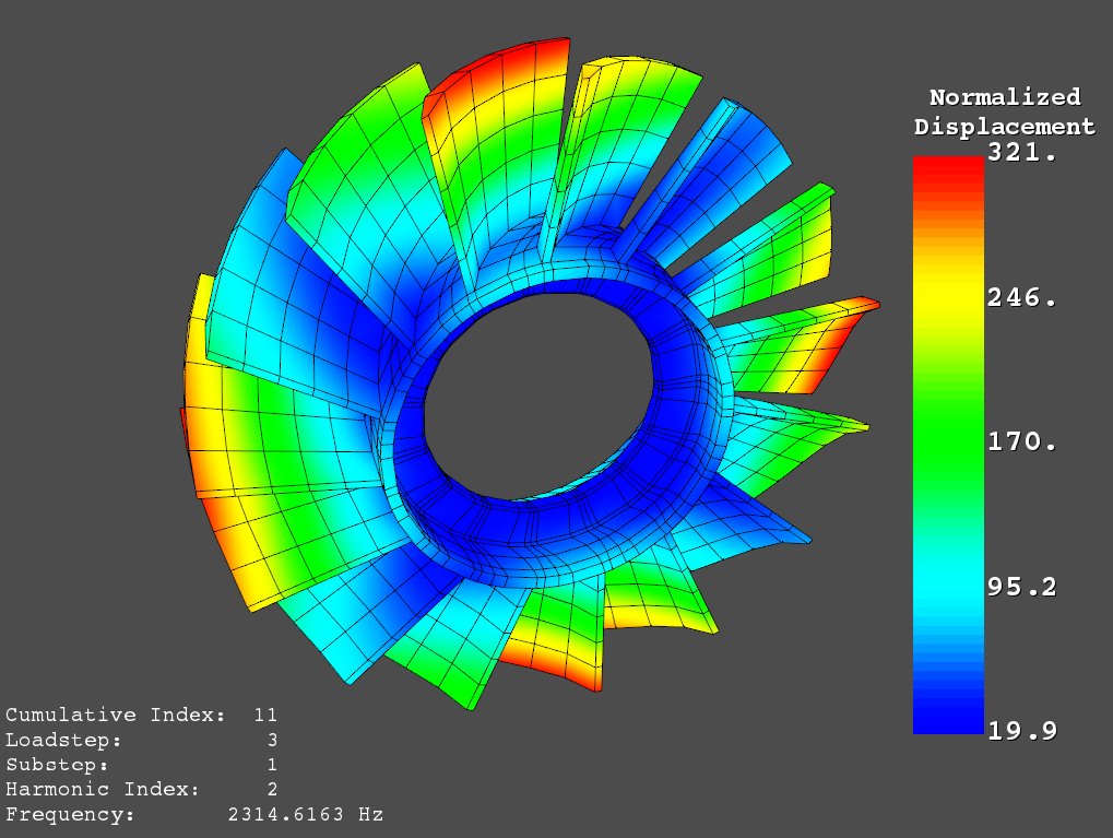
Results from a Cyclic Analysis

The ansys-mapdl-reader module can load and display the results of a cyclic analysis:

from ansys.mapdl import reader as pymapdl_reader

# load the result file
result = pymapdl_reader.read_binary('rotor.rst')

You can reference the load step table and harmonic index tables by printing the result header dictionary keys 'ls_table' and 'hindex':

>>> print(result.resultheader['ls_table'])
# load step, sub step, cumulative index
array([[ 1,  1,  1],
       [ 1,  2,  2],
       [ 1,  3,  3],
       [ 1,  4,  4],
       [ 1,  5,  5],
       [ 2,  1,  6],

>>> print(result.resultheader['hindex'])
array([0, 0, 0, 0, 0, 1, 1, 1, 1, 1, 2, 2, 2, 2, 2, 3, 3, 3, 3, 3, 4, 4, 4,
       4, 4, 5, 5, 5, 5, 5, 6, 6, 6, 6, 6, 7, 7, 7, 7, 7], dtype=int32)

Where each harmonic index entry corresponds a cumulative index. For example, result number 11 is the first mode for the 2nd harmonic index:

>>> result.resultheader['ls_table'][10] # Result 11 (using zero based indexing)
array([ 3,  1, 11], dtype=int32)

>>> result.resultheader['hindex'][10]
2

Alternatively, the result number can be obtained by using:

>>> mode = 1
>>> harmonic_index = 2
>>> result.harmonic_index_to_cumulative(mode, harmonic_index)
24

Using this indexing method, repeated modes are indexed by the same mode index. To access the other repeated mode, use a negative harmonic index. Should a result not exist, ansys-mapdl-reader will return which modes are available:

>>> mode = 1
>>> harmonic_index = 20
>>> result.harmonic_index_to_cumulative(mode, harmonic_index)
Exception: Invalid mode for harmonic index 1
Available modes: [0 1 2 3 4 5 6 7 8 9]

Results from a cyclic analysis require additional post processing to be interpreted correctly. Mode shapes are stored within the result file as unprocessed parts of the real and imaginary parts of a modal solution. ansys-mapdl-reader combines these values into a single complex array and then returns the real result of that array.

>>> nnum, ms = result.nodal_solution(10) # mode shape of result 11
>>> print(ms[:3])
[[ 44.700, 45.953, 38.717]
 [ 42.339, 48.516, 52.475]
 [ 36.000, 33.121, 39.044]]

Sometimes it is necessary to determine the maximum displacement of a mode. To do so, return the complex solution with:

nnum, ms = result.nodal_solution(0, as_complex=True)
norm = np.abs((ms*ms).sum(1)**0.5)
idx = np.nanargmax(norm)
ang = np.angle(ms[idx, 0])

# rotate the solution by the angle of the maximum nodal response
ms *= np.cos(ang) - 1j*np.sin(ang)

# get only the real response
ms = np.real(ms)

See help(result.nodal_solution) for more details.

The real displacement of the sector is always the real component of the mode shape ms, and this can be varied by multiplying the mode shape by a complex value for a given phase.

The results of a single sector can be displayed as well using the plot_nodal_solution

rnum = result.harmonic_index_to_cumulative(0, 2)
result.plot_nodal_solution(rnum, label='Displacement', expand=False)

The phase of the result can be changed by modifying the phase option. See help(result.plot_nodal_solution) for details on its implementation.

Exporting to ParaView

ParaView is a visualization application that can be used for rapid generation of plots and graphs using VTK through a GUI. ansys-mapdl-reader can translate the MAPDL result files to ParaView compatible files containing the geometry and nodal results from the analysis:

from ansys.mapdl import reader as pymapdl_reader
from ansys.mapdl.reader import examples

# load example beam result file
result = pymapdl_reader.read_binary(examples.rstfile)

# save as a binary vtk xml file
result.save_as_vtk('beam.vtu')

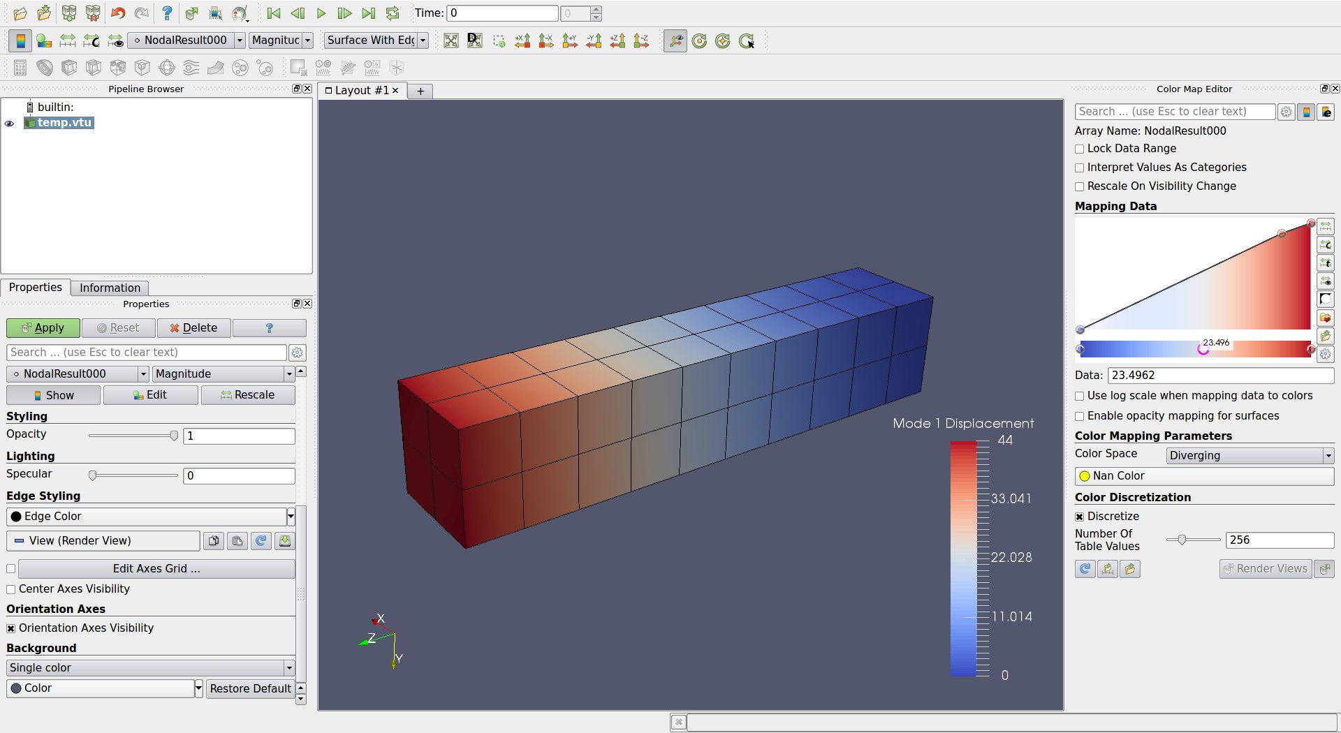
The vtk xml file can now be loaded using ParaView. This screenshot shows the nodal displacement of the first result from the result file plotted within ParaView. Within the vtk file are two point arrays (NodalResult and nodal_stress) for each result in the result file. The nodal result values will depend on the analysis type, while nodal stress will always be the node average stress in the Sx, Sy Sz, Sxy, Syz, and Sxz directions.

Result Object Methods

class ansys.mapdl.reader.rst.Result(filename, read_mesh=True, parse_vtk=True, **kwargs)

Reads a binary ANSYS result file.

Parameters:

• filename (str, pathlib.Path, optional) – Filename of the ANSYS binary result file.

• ignore_cyclic (bool, optional) – Ignores any cyclic properties.

• read_mesh (bool, optional) – Debug parameter. Set to False to disable reading in the mesh from the result file.

• parse_vtk (bool, optional) – Set to False to skip the parsing the mesh as a VTK UnstructuredGrid, which might take a long time for large models.

Examples

>>> from ansys.mapdl import reader as pymapdl_reader
>>> rst = pymapdl_reader.read_binary('file.rst')

animate_nodal_displacement(rnum, comp='norm', node_components=None, element_components=None, sel_type_all=True, add_text=True, displacement_factor=0.1, n_frames=100, loop=True, movie_filename=None, progress_bar=True, **kwargs)

Animate nodal solution.

Assumes nodal solution is a displacement array from a modal or static solution.

rnumint or list

Cumulative result number with zero based indexing, or a list containing (step, substep) of the requested result.

compstr, default: “norm”

Scalar component to display. Options are 'x', 'y', 'z', and 'norm', and None.

node_componentslist, optional

Accepts either a string or a list strings of node components to plot. For example: ['MY_COMPONENT', 'MY_OTHER_COMPONENT]

element_componentslist, optional

Accepts either a string or a list strings of element components to plot. For example: ['MY_COMPONENT', 'MY_OTHER_COMPONENT]

sel_type_allbool, optional

If node_components is specified, plots those elements containing all nodes of the component. Default True.

add_textbool, optional

Adds information about the result.

displacement_factorfloat, optional

Increases or decreases displacement by a factor.

n_framesint, optional

Number of “frames” between each full cycle.

loopbool, optional

Loop the animation. Default True. Disable this to animate once and close. Automatically disabled when off_screen=True and movie_filename is set.

movie_filenamestr, pathlib.Path, optional

Filename of the movie to open. Filename should end in 'mp4', but other filetypes may be supported like "gif". See imagio.get_writer. A single loop of the mode will be recorded.

progress_barbool, default: True

Displays a progress bar when generating a movie while off_screen=True.

kwargsoptional keyword arguments

See pyvista.plot() for additional keyword arguments.

Examples

Animate the first result interactively.

>>> rst.animate_nodal_solution(0)

Animate second result while displaying the x scalars without looping

>>> rst.animate_nodal_solution(1, comp='x', loop=False)

Animate the second result and save as a movie.

>>> rst.animate_nodal_solution(0, movie_filename='disp.mp4')

Animate the second result and save as a movie in the background.

>>> rst.animate_nodal_solution(0, movie_filename='disp.mp4', off_screen=True)

Disable plotting within the notebook.

>>> rst.animate_nodal_solution(0, notebook=False)

animate_nodal_solution(rnum, comp='norm', node_components=None, element_components=None, sel_type_all=True, add_text=True, displacement_factor=0.1, n_frames=100, loop=True, movie_filename=None, progress_bar=True, **kwargs)

Animate nodal solution.

Assumes nodal solution is a displacement array from a modal or static solution.

rnumint or list

Cumulative result number with zero based indexing, or a list containing (step, substep) of the requested result.

compstr, default: “norm”

Scalar component to display. Options are 'x', 'y', 'z', and 'norm', and None.

node_componentslist, optional

Accepts either a string or a list strings of node components to plot. For example: ['MY_COMPONENT', 'MY_OTHER_COMPONENT]

element_componentslist, optional

Accepts either a string or a list strings of element components to plot. For example: ['MY_COMPONENT', 'MY_OTHER_COMPONENT]

sel_type_allbool, optional

If node_components is specified, plots those elements containing all nodes of the component. Default True.

add_textbool, optional

Adds information about the result.

displacement_factorfloat, optional

Increases or decreases displacement by a factor.

n_framesint, optional

Number of “frames” between each full cycle.

loopbool, optional

Loop the animation. Default True. Disable this to animate once and close. Automatically disabled when off_screen=True and movie_filename is set.

movie_filenamestr, pathlib.Path, optional

Filename of the movie to open. Filename should end in 'mp4', but other filetypes may be supported like "gif". See imagio.get_writer. A single loop of the mode will be recorded.

progress_barbool, default: True

Displays a progress bar when generating a movie while off_screen=True.

kwargsoptional keyword arguments

See pyvista.plot() for additional keyword arguments.

Examples

Animate the first result interactively.

>>> rst.animate_nodal_solution(0)

Animate second result while displaying the x scalars without looping

>>> rst.animate_nodal_solution(1, comp='x', loop=False)

Animate the second result and save as a movie.

>>> rst.animate_nodal_solution(0, movie_filename='disp.mp4')

Animate the second result and save as a movie in the background.

>>> rst.animate_nodal_solution(0, movie_filename='disp.mp4', off_screen=True)

Disable plotting within the notebook.

>>> rst.animate_nodal_solution(0, notebook=False)

animate_nodal_solution_set(rnums=None, comp='norm', node_components=None, element_components=None, sel_type_all=True, loop=True, movie_filename=None, add_text=True, fps=20, **kwargs)

Animate a set of nodal solutions.

Animates the scalars of all the result sets. Best when used with a series of static analyses.

rnumscollection.Iterable

Range or list containing the zero based indexed cumulative result numbers to animate.

compstr, optional

Scalar component to display. Options are 'x', 'y', 'z', and 'norm', and None. Not applicable for a thermal analysis.

node_componentslist, optional

Accepts either a string or a list strings of node components to plot. For example: ['MY_COMPONENT', 'MY_OTHER_COMPONENT]

element_componentslist, optional

Accepts either a string or a list strings of element components to plot. For example: ['MY_COMPONENT', 'MY_OTHER_COMPONENT]

sel_type_allbool, optional

If node_components is specified, plots those elements containing all nodes of the component. Default True.

loopbool, optional

Loop the animation. Default True. Disable this to animate once and close.

movie_filenamestr, optional

Filename of the movie to open. Filename should end in 'mp4', but other filetypes may be supported. See imagio.get_writer. A single loop of the mode will be recorded.

add_textbool, optional

Adds information about the result to the animation.

fpsint, optional

Frames per second. Defaults to 20 and limited to hardware capabilities and model density. Carries over to movies created by providing the movie_filename argument, but not to gifs.

kwargsoptional keyword arguments, optional

See help(pyvista.Plot) for additional keyword arguments.

Examples

Animate all results

>>> rst.animate_nodal_solution_set()

Animate every 50th result in a set of results and save to a gif. Use the “zx” camera position to view the ZX plane from the top down.

>>> rsets = range(0, rst.nsets, 50)
>>> rst.animate_nodal_solution_set(rsets,
...                                scalar_bar_args={'title': 'My Animation'},
...                                lighting=False, cpos='zx',
...                                movie_filename='example.gif')

property available_results

Available result types.

Examples

>>> rst.available_results
Available Results:
ENS : Nodal stresses
ENG : Element energies and volume
EEL : Nodal elastic strains
EPL : Nodal plastic strains
ETH : Nodal thermal strains (includes swelling strains)
EUL : Element euler angles
ENL : Nodal nonlinear items, e.g. equivalent plastic strains
EPT : Nodal temperatures
NSL : Nodal displacements
RF  : Nodal reaction forces

cs_4x4(cs_cord, as_vtk_matrix=False)

Return a 4x4 transformation matrix for a given coordinate system.

Parameters:

• cs_cord (int) – Coordinate system index.

• as_vtk_matrix (bool, default: False) – Return the transformation matrix as a vtkMatrix4x4.

Returns:

Matrix or vtkMatrix4x4 depending on the value of as_vtk_matrix.

Return type:

np.ndarray | vtk.vtkMatrix4x4

Notes

Values 11 and greater correspond to local coordinate systems

Examples

Return the transformation matrix for coordinate system 1.

>>> tmat = rst.cs_4x4(1)
>>> tmat
array([[1., 0., 0., 0.],
       [0., 1., 0., 0.],
       [0., 0., 1., 0.],
       [0., 0., 0., 1.]])

Return the transformation matrix for coordinate system 5. This corresponds to CSYS, 5, the cylindrical with global Cartesian Y as the axis of rotation.

>>> tmat = rst.cs_4x4(5)
>>> tmat
array([[ 1.,  0.,  0.,  0.],
       [ 0.,  0., -1.,  0.],
       [ 0.,  1.,  0.,  0.],
       [ 0.,  0.,  0.,  1.]])

cylindrical_nodal_stress(rnum, nodes=None)

Retrieves the stresses for each node in the solution in the cylindrical coordinate system as the following values:

R, THETA, Z, RTHETA, THETAZ, and RZ

The order of the results corresponds to the sorted node numbering.

Computes the nodal stress by averaging the stress for each element at each node. Due to the discontinuities across elements, stresses will vary based on the element they are evaluated from.

Parameters:

• rnum (int or list) – Cumulative result number with zero based indexing, or a list containing (step, substep) of the requested result.

• nodes (str, sequence of int or str, optional) –

  Select a limited subset of nodes. Can be a nodal component or array of node numbers. For example

  • "MY_COMPONENT"

  • ['MY_COMPONENT', 'MY_OTHER_COMPONENT]

  • np.arange(1000, 2001)

Returns:

• nnum (numpy.ndarray) – Node numbers of the result.

• stress (numpy.ndarray) – Stresses at R, THETA, Z, RTHETA, THETAZ, RZ averaged at each corner node where R is radial.

Examples

>>> from ansys.mapdl import reader as pymapdl_reader
>>> rst = pymapdl_reader.read_binary('file.rst')
>>> nnum, stress = rst.cylindrical_nodal_stress(0)

Return the cylindrical nodal stress just for the nodal component 'MY_COMPONENT'.

>>> nnum, stress = rst.cylindrical_nodal_stress(0, nodes='MY_COMPONENT')

Return the nodal stress just for the nodes from 20 through 50.

>>> nnum, stress = rst.cylindrical_nodal_stress(0, nodes=range(20, 51))

Notes

Nodes without a stress value will be NAN. Equivalent ANSYS commands: RSYS, 1 PRNSOL, S

property element_components

Dictionary of ansys element components from the result file.

Examples

>>> from ansys.mapdl import reader as pymapdl_reader
>>> from ansys.mapdl.reader import examples
>>> rst = pymapdl_reader.read_binary(examples.rstfile)
>>> rst.element_components
{'ECOMP1': array([17, 18, 21, 22, 23, 24, 25, 26, 27, 28, 29,
        30, 31, 32, 33, 34, 35, 36, 37, 38, 39, 40], dtype=int32),
'ECOMP2': array([ 1, 2, 3, 4, 5, 6, 7, 8, 9, 10, 11, 12, 13,
        14, 15, 16, 17, 18, 19, 20, 23, 24], dtype=int32),
'ELEM_COMP': array([ 5, 6, 7, 8, 9, 10, 11, 12, 13, 14, 15,
        16, 17, 18, 19, 20], dtype=int32)}

element_lookup(element_id)

Index of the element the element within the result mesh

element_solution_data(rnum, datatype, sort=True, **kwargs)

Retrieves element solution data. Similar to ETABLE.

Parameters:

• rnum (int or list) – Cumulative result number with zero based indexing, or a list containing (step, substep) of the requested result.

• datatype (str) –

  Element data type to retrieve.

  • EMS: misc. data

  • ENF: nodal forces

  • ENS: nodal stresses

  • ENG: volume and energies

  • EGR: nodal gradients

  • EEL: elastic strains

  • EPL: plastic strains

  • ECR: creep strains

  • ETH: thermal strains

  • EUL: euler angles

  • EFX: nodal fluxes

  • ELF: local forces

  • EMN: misc. non-sum values

  • ECD: element current densities

  • ENL: nodal nonlinear data

  • EHC: calculated heat generations

  • EPT: element temperatures

  • ESF: element surface stresses

  • EDI: diffusion strains

  • ETB: ETABLE items

  • ECT: contact data

  • EXY: integration point locations

  • EBA: back stresses

  • ESV: state variables

  • MNL: material nonlinear record

• sort (bool) – Sort results by element number. Default True.

• **kwargs (optional keyword arguments) – Hidden options for distributed result files.

Returns:

• enum (np.ndarray) – Element numbers.

• element_data (list) – List with one data item for each element.

• enode (list) – Node numbers corresponding to each element. results. One list entry for each element.

Notes

See ANSYS element documentation for available items for each element type. See:

https://www.mm.bme.hu/~gyebro/files/ans_help_v182/ans_elem/

Examples

Retrieve “LS” solution results from an PIPE59 element for result set 1

>>> enum, edata, enode = result.element_solution_data(0, datatype='ENS')
>>> enum[0]  # first element number
>>> enode[0]  # nodes belonging to element 1
>>> edata[0]  # data belonging to element 1
array([ -4266.19   ,   -376.18857,  -8161.785  , -64706.766  ,
        -4266.19   ,   -376.18857,  -8161.785  , -45754.594  ,
        -4266.19   ,   -376.18857,  -8161.785  ,      0.     ,
        -4266.19   ,   -376.18857,  -8161.785  ,  45754.594  ,
        -4266.19   ,   -376.18857,  -8161.785  ,  64706.766  ,
        -4266.19   ,   -376.18857,  -8161.785  ,  45754.594  ,
        -4266.19   ,   -376.18857,  -8161.785  ,      0.     ,
        -4266.19   ,   -376.18857,  -8161.785  , -45754.594  ,
        -4274.038  ,   -376.62527,  -8171.2603 ,   2202.7085 ,
       -29566.24   ,   -376.62527,  -8171.2603 ,   1557.55   ,
       -40042.613  ,   -376.62527,  -8171.2603 ,      0.     ,
       -29566.24   ,   -376.62527,  -8171.2603 ,  -1557.55   ,
        -4274.038  ,   -376.62527,  -8171.2603 ,  -2202.7085 ,
        21018.164  ,   -376.62527,  -8171.2603 ,  -1557.55   ,
        31494.537  ,   -376.62527,  -8171.2603 ,      0.     ,
        21018.164  ,   -376.62527,  -8171.2603 ,   1557.55   ],
      dtype=float32)

This data corresponds to the results you would obtain directly from MAPDL with ESOL commands:

>>> ansys.esol(nvar='2', elem=enum[0], node=enode[0][0], item='LS', comp=1)
>>> ansys.vget(par='SD_LOC1', ir='2', tstrt='1') # store in a variable
>>> ansys.read_float_parameter('SD_LOC1(1)')
-4266.19

element_stress(rnum, principal=False, in_element_coord_sys=False, **kwargs)

Retrieves the element component stresses.

Equivalent ANSYS command: PRESOL, S

Parameters:

• rnum (int or list) – Cumulative result number with zero based indexing, or a list containing (step, substep) of the requested result.

• principal (bool, optional) – Returns principal stresses instead of component stresses. Default False.

• in_element_coord_sys (bool, optional) – Returns the results in the element coordinate system. Default False and will return the results in the global coordinate system.

• **kwargs (optional keyword arguments) – Hidden options for distributed result files.

Returns:

• enum (np.ndarray) – ANSYS element numbers corresponding to each element.

• element_stress (list) – Stresses at each element for each node for Sx Sy Sz Sxy Syz Sxz or SIGMA1, SIGMA2, SIGMA3, SINT, SEQV when principal is True.

• enode (list) – Node numbers corresponding to each element’s stress results. One list entry for each element.

Examples

Element component stress for the first result set.

>>> rst.element_stress(0)

Element principal stress for the first result set.

>>> enum, element_stress, enode = result.element_stress(0, principal=True)

Notes

Shell stresses for element 181 are returned for top and bottom layers. Results are ordered such that the top layer and then the bottom layer is reported.

property filename: str

String form of the filename. This property is read-only.

property materials

Result file material properties.

Returns:

Dictionary of Materials. Keys are the material numbers, and each material is a dictionary of the material properrties of that material with only the valid entries filled.

Return type:

dict

Notes

Material properties:

• EX : Elastic modulus, element x direction (Force/Area)

• EY : Elastic modulus, element y direction (Force/Area)

• EZ : Elastic modulus, element z direction (Force/Area)

• ALPX : Coefficient of thermal expansion, element x direction (Strain/Temp)

• ALPY : Coefficient of thermal expansion, element y direction (Strain/Temp)

• ALPZ : Coefficient of thermal expansion, element z direction (Strain/Temp)

• REFT : Reference temperature (as a property) [TREF]

• PRXY : Major Poisson’s ratio, x-y plane

• PRYZ : Major Poisson’s ratio, y-z plane

• PRX Z : Major Poisson’s ratio, x-z plane

• NUXY : Minor Poisson’s ratio, x-y plane

• NUYZ : Minor Poisson’s ratio, y-z plane

• NUXZ : Minor Poisson’s ratio, x-z plane

• GXY : Shear modulus, x-y plane (Force/Area)

• GYZ : Shear modulus, y-z plane (Force/Area)

• GXZ : Shear modulus, x-z plane (Force/Area)

• DAMP : K matrix multiplier for damping [BETAD] (Time)

• MUCoefficient of friction (or, for FLUID29 and FLUID30

  elements, boundary admittance)

• DENS : Mass density (Mass/Vol)

• C : Specific heat (Heat/Mass*Temp)

• ENTH : Enthalpy (e DENS*C d(Temp)) (Heat/Vol)

• KXXThermal conductivity, element x direction

  (Heat*Length / (Time*Area*Temp))

• KYYThermal conductivity, element y direction

  (Heat*Length / (Time*Area*Temp))

• KZZThermal conductivity, element z direction

  (Heat*Length / (Time*Area*Temp))

• HF : Convection (or film) coefficient (Heat / (Time*Area*Temp))

• EMIS : Emissivity

• QRATE : Heat generation rate (MASS71 element only) (Heat/Time)

• VISC : Viscosity (Force*Time / Length2)

• SONC : Sonic velocity (FLUID29 and FLUID30 elements only) (Length/Time)

• RSVX : Electrical resistivity, element x direction (Resistance*Area / Length)

• RSVY : Electrical resistivity, element y direction (Resistance*Area / Length)

• RSVZ : Electrical resistivity, element z direction (Resistance*Area / Length)

• PERX : Electric permittivity, element x direction (Charge2 / (Force*Length))

• PERY : Electric permittivity, element y direction (Charge2 / (Force*Length))

• PERZ : Electric permittivity, element z direction (Charge2 / (Force*Length))

• MURX : Magnetic relative permeability, element x direction

• MURY : Magnetic relative permeability, element y direction

• MURZ : Magnetic relative permeability, element z direction

• MGXX : Magnetic coercive force, element x direction (Charge / (Length*Time))

• MGYY : Magnetic coercive force, element y direction (Charge / (Length*Time))

• MGZZ : Magnetic coercive force, element z direction (Charge / (Length*Time))

Materials may contain the key "stress_failure_criteria", which contains failure criteria information for temperature-dependent stress limits. This includes the following keys:

• XTEN : Allowable tensile stress or strain in the x-direction. (Must be positive.)

• XCMP : Allowable compressive stress or strain in the x-direction. (Defaults to negative of XTEN.)

• YTEN : Allowable tensile stress or strain in the y-direction. (Must be positive.)

• YCMP : Allowable compressive stress or strain in the y-direction. (Defaults to negative of YTEN.)

• ZTEN : Allowable tensile stress or strain in the z-direction. (Must be positive.)

• ZCMP : Allowable compressive stress or strain in the z-direction. (Defaults to negative of ZTEN.)

• XY : Allowable XY stress or shear strain. (Must be positive.)

• YZ : Allowable YZ stress or shear strain. (Must be positive.)

• XZ : Allowable XZ stress or shear strain. (Must be positive.)

• XYCP : XY coupling coefficient (Used only if Lab1 = S). Defaults to -1.0. [1]

• YZCP : YZ coupling coefficient (Used only if Lab1 = S). Defaults to -1.0. [1]

• XZCP : XZ coupling coefficient (Used only if Lab1 = S). Defaults to -1.0. [1]

• XZIT : XZ tensile inclination parameter for Puck failure index (default = 0.0)

• XZIC : XZ compressive inclination parameter for Puck failure index (default = 0.0)

• YZIT : YZ tensile inclination parameter for Puck failure index (default = 0.0)

• YZIC : YZ compressive inclination parameter for Puck failure index (default = 0.0)

Examples

Return the material properties from the example result file. Note that the keys of rst.materials is the material type.

>>> from ansys.mapdl import reader as pymapdl_reader
>>> from ansys.mapdl.reader import examples
>>> rst = pymapdl_reader.read_binary(examples.rstfile)
>>> rst.materials
{1: {'EX': 16900000.0, 'NUXY': 0.31, 'DENS': 0.00041408}}

property mesh

Mesh from result file.

Examples

>>> rst.mesh
ANSYS Mesh
  Number of Nodes:              1448
  Number of Elements:           226
  Number of Element Types:      1
  Number of Node Components:    0
  Number of Element Components: 0

property n_results

Number of results

property n_sector

Number of sectors

nodal_acceleration(rnum, in_nodal_coord_sys=False)

Nodal velocities for a given result set.

Parameters:

• rnum (int or list) – Cumulative result number with zero based indexing, or a list containing (step, substep) of the requested result.

• in_nodal_coord_sys (bool, optional) – When True, returns results in the nodal coordinate system. Default False.

Returns:

• nnum (int np.ndarray) – Node numbers associated with the results.

• result (float np.ndarray) – Array of nodal accelerations. Array is (nnod x sumdof), the number of nodes by the number of degrees of freedom which includes numdof and nfldof

Examples

>>> from ansys.mapdl import reader as pymapdl_reader
>>> rst = pymapdl_reader.read_binary('file.rst')
>>> nnum, data = rst.nodal_acceleration(0)

Notes

Some solution results may not include results for each node. These results are removed by and the node numbers of the solution results are reflected in nnum.

nodal_boundary_conditions(rnum)

Nodal boundary conditions for a given result number.

These nodal boundary conditions are generally set with the APDL command D. For example, D, 25, UX, 0.001

Parameters:

rnum (int or list) – Cumulative result number with zero based indexing, or a list containing (step, substep) of the requested result.

Returns:

• nnum (np.ndarray) – Node numbers of the nodes with boundary conditions.

• dof (np.ndarray) – Array of indices of the degrees of freedom of the nodes with boundary conditions. See rst.result_dof for the degrees of freedom associated with each index.

• bc (np.ndarray) – Boundary conditions.

Examples

Print the boundary conditions where: - Node 3 is fixed - Node 25 has UX=0.001 - Node 26 has UY=0.0011 - Node 27 has UZ=0.0012

>>> rst.nodal_boundary_conditions(0)
(array([ 3,  3,  3, 25, 26, 27], dtype=int32),
array([1, 2, 3, 1, 2, 3], dtype=int32),
array([0.    , 0.    , 0.    , 0.001 , 0.0011, 0.0012]))

nodal_displacement(rnum, in_nodal_coord_sys=False, nodes=None)

Returns the DOF solution for each node in the global cartesian coordinate system or nodal coordinate system.

Solution may be nodal temperatures or nodal displacements depending on the type of the solution.

Parameters:

• rnum (int or list) – Cumulative result number with zero based indexing, or a list containing (step, substep) of the requested result.

• in_nodal_coord_sys (bool, optional) – When True, returns results in the nodal coordinate system. Default False.

• nodes (str, sequence of int or str, optional) –

  Select a limited subset of nodes. Can be a nodal component or array of node numbers. For example

  • "MY_COMPONENT"

  • ['MY_COMPONENT', 'MY_OTHER_COMPONENT]

  • np.arange(1000, 2001)

Returns:

• nnum (int np.ndarray) – Node numbers associated with the results.

• result (float np.ndarray) – Array of nodal displacements or nodal temperatures. Array is (nnod x sumdof), the number of nodes by the number of degrees of freedom which includes numdof and nfldof

Examples

Return the nodal solution (in this case, displacement) for the first result of "file.rst".

>>> from ansys.mapdl import reader as pymapdl_reader
>>> rst = pymapdl_reader.read_binary('file.rst')
>>> nnum, data = rst.nodal_solution(0)

Return the nodal solution just for the nodal component 'MY_COMPONENT'.

>>> nnum, data = rst.nodal_solution(0, nodes='MY_COMPONENT')

Return the nodal solution just for the nodes from 20 through 50.

>>> nnum, data = rst.nodal_solution(0, nodes=range(20, 51))

Notes

Some solution results may not include results for each node. These results are removed by and the node numbers of the solution results are reflected in nnum.

nodal_elastic_strain(rnum, nodes=None)

Nodal component elastic strains. This record contains strains in the order X, Y, Z, XY, YZ, XZ, EQV.

Elastic strains can be can be nodal values extrapolated from the integration points or values at the integration points moved to the nodes.

Equivalent MAPDL command: PRNSOL, EPEL

Parameters:

• rnum (int or list) – Cumulative result number with zero based indexing, or a list containing (step, substep) of the requested result.

• nodes (str, sequence of int or str, optional) –

  Select a limited subset of nodes. Can be a nodal component or array of node numbers. For example

  • "MY_COMPONENT"

  • ['MY_COMPONENT', 'MY_OTHER_COMPONENT]

  • np.arange(1000, 2001)

Returns:

• nnum (np.ndarray) – MAPDL node numbers.

• elastic_strain (np.ndarray) – Nodal component elastic strains. Array is in the order X, Y, Z, XY, YZ, XZ, EQV.

Examples

Load the nodal elastic strain for the first result.

>>> from ansys.mapdl import reader as pymapdl_reader
>>> rst = pymapdl_reader.read_binary('file.rst')
>>> nnum, elastic_strain = rst.nodal_elastic_strain(0)

Return the nodal elastic strain just for the nodal component 'MY_COMPONENT'.

>>> nnum, elastic_strain = rst.nodal_elastic_strain(0, nodes='MY_COMPONENT')

Return the nodal elastic strain just for the nodes from 20 through 50.

>>> nnum, elastic_strain = rst.nodal_elastic_strain(0, nodes=range(20, 51))

Notes

Nodes without a strain will be NAN.

nodal_input_force(rnum)

Nodal input force for a given result number.

Nodal input force is generally set with the APDL command F. For example, F, 25, FX, 0.001

Parameters:

rnum (int or list) – Cumulative result number with zero based indexing, or a list containing (step, substep) of the requested result.

Returns:

• nnum (np.ndarray) – Node numbers of the nodes with nodal forces.

• dof (np.ndarray) – Array of indices of the degrees of freedom of the nodes with input force. See rst.result_dof for the degrees of freedom associated with each index.

• force (np.ndarray) – Nodal input force.

Examples

Print the nodal input force where: - Node 25 has FX=20 - Node 26 has FY=30 - Node 27 has FZ=40

>>> rst.nodal_input_force(0)
(array([ 71,  52, 127], dtype=int32),
 array([2, 1, 3], dtype=int32),
 array([30., 20., 40.]))

nodal_plastic_strain(rnum, nodes=None)

Nodal component plastic strains.

This record contains strains in the order: X, Y, Z, XY, YZ, XZ, EQV.

Plastic strains are always values at the integration points moved to the nodes.

Parameters:

• rnum (int or list) – Cumulative result number with zero based indexing, or a list containing (step, substep) of the requested result.

• nodes (str, sequence of int or str, optional) –

  Select a limited subset of nodes. Can be a nodal component or array of node numbers. For example

  • "MY_COMPONENT"

  • ['MY_COMPONENT', 'MY_OTHER_COMPONENT]

  • np.arange(1000, 2001)

Returns:

• nnum (np.ndarray) – MAPDL node numbers.

• plastic_strain (np.ndarray) – Nodal component plastic strains. Array is in the order X, Y, Z, XY, YZ, XZ, EQV.

Examples

Load the nodal plastic strain for the first solution.

>>> from ansys.mapdl import reader as pymapdl_reader
>>> rst = pymapdl_reader.read_binary('file.rst')
>>> nnum, plastic_strain = rst.nodal_plastic_strain(0)

Return the nodal plastic strain just for the nodal component 'MY_COMPONENT'.

>>> nnum, plastic_strain = rst.nodal_plastic_strain(0, nodes='MY_COMPONENT')

Return the nodal plastic strain just for the nodes from 20 through 50.

>>> nnum, plastic_strain = rst.nodal_plastic_strain(0, nodes=range(20, 51))

nodal_reaction_forces(rnum)

Nodal reaction forces.

Parameters:

rnum (int or list) – Cumulative result number with zero based indexing, or a list containing (step, substep) of the requested result.

Returns:

• rforces (np.ndarray) – Nodal reaction forces for each degree of freedom.

• nnum (np.ndarray) – Node numbers corresponding to the reaction forces. Node numbers may be repeated if there is more than one degree of freedom for each node.

• dof (np.ndarray) – Degree of freedom corresponding to each node using the MAPDL degree of freedom reference table. See rst.result_dof for the corresponding degrees of freedom for a given solution.

Examples

Get the nodal reaction forces for the first result and print the reaction forces of a single node.

>>> from ansys.mapdl import reader as pymapdl_reader
>>> rst = pymapdl_reader.read_binary('file.rst')
>>> rforces, nnum, dof = rst.nodal_reaction_forces(0)
>>> dof_ref = rst.result_dof(0)
>>> rforces[:3], nnum[:3], dof[:3], dof_ref
(array([  24102.21376091, -109357.01854005,   22899.5303263 ]),
 array([4142, 4142, 4142]),
 array([1, 2, 3], dtype=int32),
 ['UX', 'UY', 'UZ'])

nodal_solution(rnum, in_nodal_coord_sys=False, nodes=None)

Returns the DOF solution for each node in the global cartesian coordinate system or nodal coordinate system.

Solution may be nodal temperatures or nodal displacements depending on the type of the solution.

Parameters:

• rnum (int or list) – Cumulative result number with zero based indexing, or a list containing (step, substep) of the requested result.

• in_nodal_coord_sys (bool, optional) – When True, returns results in the nodal coordinate system. Default False.

• nodes (str, sequence of int or str, optional) –

  Select a limited subset of nodes. Can be a nodal component or array of node numbers. For example

  • "MY_COMPONENT"

  • ['MY_COMPONENT', 'MY_OTHER_COMPONENT]

  • np.arange(1000, 2001)

Returns:

• nnum (int np.ndarray) – Node numbers associated with the results.

• result (float np.ndarray) – Array of nodal displacements or nodal temperatures. Array is (nnod x sumdof), the number of nodes by the number of degrees of freedom which includes numdof and nfldof

Examples

Return the nodal solution (in this case, displacement) for the first result of "file.rst".

>>> from ansys.mapdl import reader as pymapdl_reader
>>> rst = pymapdl_reader.read_binary('file.rst')
>>> nnum, data = rst.nodal_solution(0)

Return the nodal solution just for the nodal component 'MY_COMPONENT'.

>>> nnum, data = rst.nodal_solution(0, nodes='MY_COMPONENT')

Return the nodal solution just for the nodes from 20 through 50.

>>> nnum, data = rst.nodal_solution(0, nodes=range(20, 51))

Notes

Some solution results may not include results for each node. These results are removed by and the node numbers of the solution results are reflected in nnum.

nodal_static_forces(rnum, nodes=None)

Return the nodal forces averaged at the nodes.

Nodal forces are computed on an element by element basis, and this method averages the nodal forces for each element for each node.

Parameters:

• rnum (int or list) – Cumulative result number with zero based indexing, or a list containing (step, substep) of the requested result.

• nodes (str, sequence of int or str, optional) –

  Select a limited subset of nodes. Can be a nodal component or array of node numbers. For example

  • "MY_COMPONENT"

  • ['MY_COMPONENT', 'MY_OTHER_COMPONENT]

  • np.arange(1000, 2001)

Returns:

• nnum (np.ndarray) – MAPDL node numbers.

• forces (np.ndarray) – Averaged nodal forces. Array is sized [nnod x numdof] where nnod is the number of nodes and numdof is the number of degrees of freedom for this solution.

Examples

Load the nodal static forces for the first result using the example hexahedral result file.

>>> from ansys.mapdl import reader as pymapdl_reader
>>> from ansys.mapdl.reader import examples
>>> rst = pymapdl_reader.read_binary(examples.rstfile)
>>> nnum, forces = rst.nodal_static_forces(0)

Return the nodal static forces just for the nodal component 'MY_COMPONENT'.

>>> nnum, forces = rst.nodal_static_forces(0, nodes='MY_COMPONENT')

Return the nodal static forces just for the nodes from 20 through 50.

>>> nnum, forces = rst.nodal_static_forces(0, nodes=range(20, 51))

Notes

Nodes without a a nodal will be NAN. These are generally midside (quadratic) nodes.

nodal_stress(rnum, nodes=None)

Retrieves the component stresses for each node in the solution.

The order of the results corresponds to the sorted node numbering.

Computes the nodal stress by averaging the stress for each element at each node. Due to the discontinuities across elements, stresses will vary based on the element they are evaluated from.

Parameters:

• rnum (int or list) – Cumulative result number with zero based indexing, or a list containing (step, substep) of the requested result.

• nodes (str, sequence of int or str, optional) –

  Select a limited subset of nodes. Can be a nodal component or array of node numbers. For example

  • "MY_COMPONENT"

  • ['MY_COMPONENT', 'MY_OTHER_COMPONENT]

  • np.arange(1000, 2001)

Returns:

• nnum (numpy.ndarray) – Node numbers of the result.

• stress (numpy.ndarray) – Stresses at X, Y, Z, XY, YZ, XZ averaged at each corner node.

Examples

>>> from ansys.mapdl import reader as pymapdl_reader
>>> rst = pymapdl_reader.read_binary('file.rst')
>>> nnum, stress = rst.nodal_stress(0)

Return the nodal stress just for the nodal component 'MY_COMPONENT'.

>>> nnum, stress = rst.nodal_stress(0, nodes='MY_COMPONENT')

Return the nodal stress just for the nodes from 20 through 50.

>>> nnum, stress = rst.nodal_solution(0, nodes=range(20, 51))

Notes

Nodes without a stress value will be NAN. Equivalent ANSYS command: PRNSOL, S

nodal_temperature(rnum, nodes=None, **kwargs)

Retrieves the temperature for each node in the solution.

The order of the results corresponds to the sorted node numbering.

Equivalent MAPDL command: PRNSOL, TEMP

Parameters:

• rnum (int or list) – Cumulative result number with zero based indexing, or a list containing (step, substep) of the requested result.

• nodes (str, sequence of int or str, optional) –

  Select a limited subset of nodes. Can be a nodal component or array of node numbers. For example

  • "MY_COMPONENT"

  • ['MY_COMPONENT', 'MY_OTHER_COMPONENT]

  • np.arange(1000, 2001)

Returns:

• nnum (numpy.ndarray) – Node numbers of the result.

• temperature (numpy.ndarray) – Temperature at each node.

Examples

>>> from ansys.mapdl import reader as pymapdl_reader
>>> rst = pymapdl_reader.read_binary('file.rst')
>>> nnum, temp = rst.nodal_temperature(0)

Return the temperature just for the nodal component 'MY_COMPONENT'.

>>> nnum, temp = rst.nodal_stress(0, nodes='MY_COMPONENT')

Return the temperature just for the nodes from 20 through 50.

>>> nnum, temp = rst.nodal_solution(0, nodes=range(20, 51))

nodal_thermal_strain(rnum, nodes=None)

Nodal component thermal strain.

This record contains strains in the order X, Y, Z, XY, YZ, XZ, EQV, and eswell (element swelling strain). Thermal strains are always values at the integration points moved to the nodes.

Equivalent MAPDL command: PRNSOL, EPTH, COMP

Parameters:

• rnum (int or list) – Cumulative result number with zero based indexing, or a list containing (step, substep) of the requested result.

• nodes (str, sequence of int or str, optional) –

  Select a limited subset of nodes. Can be a nodal component or array of node numbers. For example

  • "MY_COMPONENT"

  • ['MY_COMPONENT', 'MY_OTHER_COMPONENT]

  • np.arange(1000, 2001)

Returns:

• nnum (np.ndarray) – MAPDL node numbers.

• thermal_strain (np.ndarray) – Nodal component plastic strains. Array is in the order X, Y, Z, XY, YZ, XZ, EQV, ESWELL

Examples

Load the nodal thermal strain for the first solution.

>>> from ansys.mapdl import reader as pymapdl_reader
>>> rst = pymapdl_reader.read_binary('file.rst')
>>> nnum, thermal_strain = rst.nodal_thermal_strain(0)

Return the nodal thermal strain just for the nodal component 'MY_COMPONENT'.

>>> nnum, thermal_strain = rst.nodal_thermal_strain(0, nodes='MY_COMPONENT')

Return the nodal thermal strain just for the nodes from 20 through 50.

>>> nnum, thermal_strain = rst.nodal_thermal_strain(0, nodes=range(20, 51))

nodal_time_history(solution_type='NSL', in_nodal_coord_sys=False)

The DOF solution for each node for all result sets.

The nodal results are returned returned in the global cartesian coordinate system or nodal coordinate system.

Parameters:

• solution_type (str, optional) – The solution type. Must be either nodal displacements ('NSL'), nodal velocities ('VEL') or nodal accelerations ('ACC').

• in_nodal_coord_sys (bool, optional) – When True, returns results in the nodal coordinate system. Default False.

Returns:

• nnum (int np.ndarray) – Node numbers associated with the results.

• result (float np.ndarray) – Nodal solution for all result sets. Array is sized rst.nsets x nnod x Sumdof, which is the number of time steps by number of nodes by degrees of freedom.

nodal_velocity(rnum, in_nodal_coord_sys=False)

Nodal velocities for a given result set.

Parameters:

• rnum (int or list) – Cumulative result number with zero based indexing, or a list containing (step, substep) of the requested result.

• in_nodal_coord_sys (bool, optional) – When True, returns results in the nodal coordinate system. Default False.

Returns:

• nnum (int np.ndarray) – Node numbers associated with the results.

• result (float np.ndarray) – Array of nodal velocities. Array is (nnod x sumdof), the number of nodes by the number of degrees of freedom which includes numdof and nfldof

Examples

>>> from ansys.mapdl import reader as pymapdl_reader
>>> rst = pymapdl_reader.read_binary('file.rst')
>>> nnum, data = rst.nodal_velocity(0)

Notes

Some solution results may not include results for each node. These results are removed by and the node numbers of the solution results are reflected in nnum.

property node_components

Dictionary of ansys node components from the result file.

Examples

>>> from ansys.mapdl import reader as pymapdl_reader
>>> from ansys.mapdl.reader import examples
>>> rst = pymapdl_reader.read_binary(examples.rstfile)
>>> rst.node_components.keys()
dict_keys(['ECOMP1', 'ECOMP2', 'ELEM_COMP'])
>>> rst.node_components['NODE_COMP']
array([ 5, 6, 7, 8, 9, 10, 11, 12, 13, 14, 15, 16, 17, 18, 19,
      20], dtype=int32)

overwrite_element_solution_record(data, rnum, solution_type, element_id)

Overwrite element solution record.

This method replaces solution data for of an element at a result index for a given solution type. The number of items in data must match the number of items in the record.

If you are not sure how many records are in a given record, use element_solution_data to retrieve all the records for a given solution_type and check the number of items in the record.

Note: The record being replaced cannot be a compressed record. If the result file uses compression (default sparse compression as of 2019R1), you can disable this within MAPDL with: /FCOMP, RST, 0

Parameters:

• data (list or np.ndarray) – Data that will replace the existing records.

• rnum (int) – Zero based result number.

• solution_type (str) –

  Element data type to overwrite.

  • EMS: misc. data

  • ENF: nodal forces

  • ENS: nodal stresses

  • ENG: volume and energies

  • EGR: nodal gradients

  • EEL: elastic strains

  • EPL: plastic strains

  • ECR: creep strains

  • ETH: thermal strains

  • EUL: euler angles

  • EFX: nodal fluxes

  • ELF: local forces

  • EMN: misc. non-sum values

  • ECD: element current densities

  • ENL: nodal nonlinear data

  • EHC: calculated heat generations

  • EPT: element temperatures

  • ESF: element surface stresses

  • EDI: diffusion strains

  • ETB: ETABLE items

  • ECT: contact data

  • EXY: integration point locations

  • EBA: back stresses

  • ESV: state variables

  • MNL: material nonlinear record

• element_id (int) – Ansys element number (e.g. 1)

Examples

Overwrite the elastic strain record for element 1 for the first result with random data.

>>> from ansys.mapdl import reader as pymapdl_reader
>>> rst = pymapdl_reader.read_binary('file.rst')
>>> data = np.random.random(56)
>>> rst.overwrite_element_solution_data(data, 0, 'EEL', 1)

overwrite_element_solution_records(element_data, rnum, solution_type)

Overwrite element solution record.

This method replaces solution data for a set of elements at a result index for a given solution type. The number of items in data must match the number of items in the record.

If you are not sure how many records are in a given record, use element_solution_data to retrieve all the records for a given solution_type and check the number of items in the record.

Note: The record being replaced cannot be a compressed record. If the result file uses compression (default sparse compression as of 2019R1), you can disable this within MAPDL with: /FCOMP, RST, 0

Parameters:

• element_data (dict) – Dictionary of results that will replace the existing records.

• rnum (int) – Zero based result number.

• solution_type (str) –

  Element data type to overwrite.

  • EMS: misc. data

  • ENF: nodal forces

  • ENS: nodal stresses

  • ENG: volume and energies

  • EGR: nodal gradients

  • EEL: elastic strains

  • EPL: plastic strains

  • ECR: creep strains

  • ETH: thermal strains

  • EUL: euler angles

  • EFX: nodal fluxes

  • ELF: local forces

  • EMN: misc. non-sum values

  • ECD: element current densities

  • ENL: nodal nonlinear data

  • EHC: calculated heat generations

  • EPT: element temperatures

  • ESF: element surface stresses

  • EDI: diffusion strains

  • ETB: ETABLE items

  • ECT: contact data

  • EXY: integration point locations

  • EBA: back stresses

  • ESV: state variables

  • MNL: material nonlinear record

Examples

Overwrite the elastic strain record for elements 1 and 2 with for the first result with random data.

>>> from ansys.mapdl import reader as pymapdl_reader
>>> rst = pymapdl_reader.read_binary('file.rst')
>>> data = {1: np.random.random(56),
            2: np.random.random(56)}
>>> rst.overwrite_element_solution_data(data, 0, 'EEL')

parse_coordinate_system()

Reads in coordinate system information from a binary result file.

Returns:

c_systems – Dictionary containing one entry for each defined coordinate system. If no non-standard coordinate systems have been defined, an empty dictionary will be returned. First coordinate system is assumed to be global cartesian.

Return type:

dict

Notes

euler angles : [THXY, THYZ, THZX]

• First rotation about local Z (positive X toward Y).

• Second rotation about local X (positive Y toward Z).

• Third rotation about local Y (positive Z toward X).

PAR1 Used for elliptical, spheroidal, or toroidal systems. If KCS = 1 or 2, PAR1 is the ratio of the ellipse Y-axis radius to X-axis radius (defaults to 1.0 (circle)). If KCS = 3, PAR1 is the major radius of the torus.

PAR2 Used for spheroidal systems. If KCS = 2, PAR2 = ratio of ellipse Z-axis radius to X-axis radius (defaults to 1.0 (circle)).

Coordinate system type:

• 0: Cartesian

• 1: Cylindrical (circular or elliptical)

• 2: Spherical (or spheroidal)

• 3: Toroidal

parse_step_substep(user_input)

Converts (step, substep) to a cumulative index

property pathlib_filename: Path

Return the pathlib.Path version of the filename. This property can not be set.

plot(node_components=None, element_components=None, sel_type_all=True, **kwargs)

Plot result geometry

Parameters:

• node_components (list, optional) – Accepts either a string or a list strings of node components to plot. For example: ['MY_COMPONENT', 'MY_OTHER_COMPONENT]

• element_components (list, optional) – Accepts either a string or a list strings of element components to plot. For example: ['MY_COMPONENT', 'MY_OTHER_COMPONENT]

• sel_type_all (bool, optional) – If node_components is specified, plots those elements containing all nodes of the component. Default True.

• **kwargs (keyword arguments) – Optional keyword arguments. See help(pyvista.plot).

Returns:

cpos – List of camera position, focal point, and view up.

Return type:

list

Examples

>>> from ansys.mapdl import reader as pymapdl_reader
>>> rst = pymapdl_reader.read_binary('file.rst')
>>> rst.plot()

Plot just the element component ‘ROTOR_SHAFT’

>>> rst.plot(element_components='ROTOR_SHAFT')

Plot two node components >>> rst.plot(node_components=[‘MY_COMPONENT’, ‘MY_OTHER_COMPONENT’])

plot_cylindrical_nodal_stress(rnum, comp=None, show_displacement=False, displacement_factor=1, node_components=None, element_components=None, sel_type_all=True, treat_nan_as_zero=False, **kwargs)

Plot nodal_stress in the cylindrical coordinate system.

Parameters:

• rnum (int) – Result number

• comp (str, optional) – Stress component to display. Available options: - "R" - "THETA" - "Z" - "RTHETA" - "THETAZ" - "RZ"

• show_displacement (bool, optional) – Deforms mesh according to the result.

• displacement_factor (float, optional) – Increases or decreases displacement by a factor.

• node_components (list, optional) – Accepts either a string or a list strings of node components to plot. For example: ['MY_COMPONENT', 'MY_OTHER_COMPONENT]

• element_components (list, optional) – Accepts either a string or a list strings of element components to plot. For example: ['MY_COMPONENT', 'MY_OTHER_COMPONENT]

• sel_type_all (bool, optional) – If node_components is specified, plots those elements containing all nodes of the component. Default True.

• treat_nan_as_zero (bool, optional) – Treat NAN values (i.e. stresses at midside nodes) as zero when plotting.

• **kwargs (keyword arguments) – Optional keyword arguments. See help(pyvista.plot)

Examples

Plot nodal stress in the radial direction.

>>> from ansys.mapdl import reader as pymapdl_reader
>>> result = pymapdl_reader.read_binary('file.rst')
>>> result.plot_cylindrical_nodal_stress(0, 'R')

plot_element_result(rnum, result_type, item_index, in_element_coord_sys=False, **kwargs)

Plot an element result.

Parameters:

• rnum (int) – Result number.

• result_type (str) –

  Element data type to retrieve.

  • EMS: misc. data

  • ENF: nodal forces

  • ENS: nodal stresses

  • ENG: volume and energies

  • EGR: nodal gradients

  • EEL: elastic strains

  • EPL: plastic strains

  • ECR: creep strains

  • ETH: thermal strains

  • EUL: euler angles

  • EFX: nodal fluxes

  • ELF: local forces

  • EMN: misc. non-sum values

  • ECD: element current densities

  • ENL: nodal nonlinear data

  • EHC: calculated heat generations

  • EPT: element temperatures

  • ESF: element surface stresses

  • EDI: diffusion strains

  • ETB: ETABLE items

  • ECT: contact data

  • EXY: integration point locations

  • EBA: back stresses

  • ESV: state variables

  • MNL: material nonlinear record

• item_index (int) – Index of the data item for each node within the element.

• in_element_coord_sys (bool, optional) – Returns the results in the element coordinate system. Default False and will return the results in the global coordinate system.

Returns:

• nnum (np.ndarray) – ANSYS node numbers

• result (np.ndarray) – Array of result data

plot_nodal_displacement(rnum, comp=None, show_displacement=False, displacement_factor=1.0, node_components=None, element_components=None, sel_type_all=True, treat_nan_as_zero=False, **kwargs)

Plots the nodal solution.

Parameters:

• rnum (int or list) – Cumulative result number with zero based indexing, or a list containing (step, substep) of the requested result.

• comp (str, optional) – Display component to display. Options are 'X', 'Y', 'Z', 'NORM', or an available degree of freedom. Result may also include other degrees of freedom, check rst.result_dof for available degrees of freedoms for a given result. Defaults to "NORM" for a structural displacement result, and "TEMP" for a thermal result.

• show_displacement (bool, optional) – Deforms mesh according to the result.

• displacement_factor (float, optional) – Increases or decreases displacement by a factor.

• node_components (list, optional) – Accepts either a string or a list strings of node components to plot. For example: ['MY_COMPONENT', 'MY_OTHER_COMPONENT]

• element_components (list, optional) – Accepts either a string or a list strings of element components to plot. For example: ['MY_COMPONENT', 'MY_OTHER_COMPONENT]

• sel_type_all (bool, optional) – If node_components is specified, plots those elements containing all nodes of the component. Default True.

• treat_nan_as_zero (bool, optional) – Treat NAN values (i.e. stresses at midside nodes) as zero when plotting.

• **kwargs (keyword arguments) – Optional keyword arguments. See help(pyvista.plot).

Returns:

cpos – Camera position from vtk render window.

Return type:

list

Examples

Plot the nodal solution result 0 of verification manual example

>>> from ansys.mapdl import reader as pymapdl_reader
>>> from ansys.mapdl.reader import examples
>>> result = examples.download_verification_result(33)
>>> result.plot_nodal_solution(0)

Plot with a white background and showing edges

>>> result.plot_nodal_solution(0, background='w', show_edges=True)

plot_nodal_elastic_strain(rnum, comp, scalar_bar_args={'title': 'EQV Nodal Elastic Strain'}, show_displacement=False, displacement_factor=1, node_components=None, element_components=None, sel_type_all=True, treat_nan_as_zero=False, **kwargs)

Plot nodal elastic strain.

Parameters:

• rnum (int) – Result number

• comp (str, optional) – Elastic strain component to display. Available options: - "X" - "Y" - "Z" - "XY" - "YZ" - "XZ" - "EQV"

• show_displacement (bool, optional) – Deforms mesh according to the result.

• displacement_factor (float, optional) – Increases or decreases displacement by a factor.

• node_components (list, optional) – Accepts either a string or a list strings of node components to plot. For example: ['MY_COMPONENT', 'MY_OTHER_COMPONENT']

• element_components (list, optional) – Accepts either a string or a list strings of element components to plot. For example: ['MY_COMPONENT', 'MY_OTHER_COMPONENT']

• sel_type_all (bool, optional) – If node_components is specified, plots those elements containing all nodes of the component. Default True.

• treat_nan_as_zero (bool, optional) – Treat NAN values (i.e. stresses at midside nodes) as zero when plotting.

• **kwargs (keyword arguments) – Optional keyword arguments. See help(pyvista.plot)

Examples

Plot nodal elastic strain for a static pontoon model

>>> from ansys.mapdl import reader as pymapdl_reader
>>> from ansys.mapdl.reader import examples
>>> result = examples.download_pontoon()
>>> result.plot_nodal_elastic_strain(0)

plot_nodal_plastic_strain(rnum, comp, scalar_bar_args={'title': 'Nodal Plastic Strain'}, show_displacement=False, displacement_factor=1, node_components=None, element_components=None, sel_type_all=True, treat_nan_as_zero=False, **kwargs)

Plot nodal component plastic strain.

Parameters:

• rnum (int or list) – Cumulative result number with zero based indexing, or a list containing (step, substep) of the requested result.

• comp (str, optional) – Plastic strain component to display. Available options: - "X" - "Y" - "Z" - "XY" - "YZ" - "XZ" - "EQV"

• show_displacement (bool, optional) – Deforms mesh according to the result.

• displacement_factor (float, optional) – Increases or decreases displacement by a factor.

• node_components (list, optional) – Accepts either a string or a list strings of node components to plot. For example: ['MY_COMPONENT', 'MY_OTHER_COMPONENT]

• element_components (list, optional) – Accepts either a string or a list strings of element components to plot. For example: ['MY_COMPONENT', 'MY_OTHER_COMPONENT]

• sel_type_all (bool, optional) – If node_components is specified, plots those elements containing all nodes of the component. Default True.

• treat_nan_as_zero (bool, optional) – Treat NAN values (i.e. stresses at midside nodes) as zero when plotting.

• **kwargs (keyword arguments) – Optional keyword arguments. See help(pyvista.plot).

Examples

Plot plastic strain for a static pontoon model

>>> from ansys.mapdl import reader as pymapdl_reader
>>> from ansys.mapdl.reader import examples
>>> result = examples.download_pontoon()
>>> result.plot_nodal_plastic_strain(0)

plot_nodal_solution(rnum, comp=None, show_displacement=False, displacement_factor=1.0, node_components=None, element_components=None, sel_type_all=True, treat_nan_as_zero=False, **kwargs)

Plots the nodal solution.

Parameters:

• rnum (int or list) – Cumulative result number with zero based indexing, or a list containing (step, substep) of the requested result.

• comp (str, optional) – Display component to display. Options are 'X', 'Y', 'Z', 'NORM', or an available degree of freedom. Result may also include other degrees of freedom, check rst.result_dof for available degrees of freedoms for a given result. Defaults to "NORM" for a structural displacement result, and "TEMP" for a thermal result.

• show_displacement (bool, optional) – Deforms mesh according to the result.

• displacement_factor (float, optional) – Increases or decreases displacement by a factor.

• node_components (list, optional) – Accepts either a string or a list strings of node components to plot. For example: ['MY_COMPONENT', 'MY_OTHER_COMPONENT]

• element_components (list, optional) – Accepts either a string or a list strings of element components to plot. For example: ['MY_COMPONENT', 'MY_OTHER_COMPONENT]

• sel_type_all (bool, optional) – If node_components is specified, plots those elements containing all nodes of the component. Default True.

• treat_nan_as_zero (bool, optional) – Treat NAN values (i.e. stresses at midside nodes) as zero when plotting.

• **kwargs (keyword arguments) – Optional keyword arguments. See help(pyvista.plot).

Returns:

cpos – Camera position from vtk render window.

Return type:

list

Examples

Plot the nodal solution result 0 of verification manual example

>>> from ansys.mapdl import reader as pymapdl_reader
>>> from ansys.mapdl.reader import examples
>>> result = examples.download_verification_result(33)
>>> result.plot_nodal_solution(0)

Plot with a white background and showing edges

>>> result.plot_nodal_solution(0, background='w', show_edges=True)

plot_nodal_stress(rnum, comp=None, show_displacement=False, displacement_factor=1, node_components=None, element_components=None, sel_type_all=True, treat_nan_as_zero=False, **kwargs)

Plots the stresses at each node in the solution.

Parameters:

• rnum (int or list) – Cumulative result number with zero based indexing, or a list containing (step, substep) of the requested result.

• comp (str, optional) – Stress component to display. Available options: - "X" - "Y" - "Z" - "XY" - "YZ" - "XZ"

• node_components (list, optional) – Accepts either a string or a list strings of node components to plot. For example: ['MY_COMPONENT', 'MY_OTHER_COMPONENT]

• element_components (list, optional) – Accepts either a string or a list strings of element components to plot. For example: ['MY_COMPONENT', 'MY_OTHER_COMPONENT]

• sel_type_all (bool, optional) – If node_components is specified, plots those elements containing all nodes of the component. Default True.

• treat_nan_as_zero (bool, optional) – Treat NAN values (i.e. stresses at midside nodes) as zero when plotting.

• kwargs (keyword arguments) – Additional keyword arguments. See help(pyvista.plot)

Returns:

cpos – 3 x 3 vtk camera position.

Return type:

list

Examples

Plot the X component nodal stress while showing displacement.

>>> rst.plot_nodal_stress(0, comp='x', show_displacement=True)

plot_nodal_temperature(rnum, show_displacement=False, displacement_factor=1, node_components=None, element_components=None, sel_type_all=True, treat_nan_as_zero=False, **kwargs)

Plot nodal temperature

Parameters:

• rnum (int) – Result number

• show_displacement (bool, optional) – Deforms mesh according to the result.

• displacement_factor (float, optional) – Increases or decreases displacement by a factor.

• node_components (list, optional) – Accepts either a string or a list strings of node components to plot. For example: ['MY_COMPONENT', 'MY_OTHER_COMPONENT]

• element_components (list, optional) – Accepts either a string or a list strings of element components to plot. For example: ['MY_COMPONENT', 'MY_OTHER_COMPONENT]

• sel_type_all (bool, optional) – If node_components is specified, plots those elements containing all nodes of the component. Default True.

• treat_nan_as_zero (bool, optional) – Treat NAN values (i.e. stresses at midside nodes) as zero when plotting.

• **kwargs (keyword arguments) – Optional keyword arguments. See help(pyvista.plot)

Examples

Plot temperature of a result.

>>> from ansys.mapdl import reader as pymapdl_reader
>>> result = pymapdl_reader.read_binary('file.rst')
>>> result.plot_nodal_temperature(0)

Plot while showing edges and disabling lighting

>>> result.plot_nodal_temperature(0, show_edges=True, lighting=False)

plot_nodal_thermal_strain(rnum, comp=None, scalar_bar_args={'title': 'Nodal Thermal Strain'}, show_displacement=False, displacement_factor=1, node_components=None, element_components=None, sel_type_all=True, treat_nan_as_zero=False, **kwargs)

Plot nodal component thermal strains.

Equivalent MAPDL command: PLNSOL, EPTH, COMP

Parameters:

• rnum (int) – Result number

• comp (str, optional) – Thermal strain component to display. Available options: - "X" - "Y" - "Z" - "XY" - "YZ" - "XZ" - "EQV" - "ESWELL"

• show_displacement (bool, optional) – Deforms mesh according to the result.

• displacement_factor (float, optional) – Increases or decreases displacement by a factor.

• node_components (list, optional) – Accepts either a string or a list strings of node components to plot. For example: ['MY_COMPONENT', 'MY_OTHER_COMPONENT]

• element_components (list, optional) – Accepts either a string or a list strings of element components to plot. For example: ['MY_COMPONENT', 'MY_OTHER_COMPONENT]

• sel_type_all (bool, optional) – If node_components is specified, plots those elements containing all nodes of the component. Default True.

• treat_nan_as_zero (bool, optional) – Treat NAN values (i.e. stresses at midside nodes) as zero when plotting.

• **kwargs (keyword arguments) – Optional keyword arguments. See help(pyvista.plot)

Examples

Plot thermal strain for result 0 of verification manual example 33.

>>> from ansys.mapdl import reader as pymapdl_reader
>>> from ansys.mapdl.reader import examples
>>> result = examples.download_verification_result(33)
>>> result.plot_nodal_thermal_strain(0)

plot_principal_nodal_stress(rnum, comp=None, show_displacement=False, displacement_factor=1.0, node_components=None, element_components=None, sel_type_all=True, treat_nan_as_zero=False, **kwargs)

Plot the principal stress.

Parameters:

• rnum (int or list) – Cumulative result number with zero based indexing, or a list containing (step, substep) of the requested result.

• comp (string) –

  Stress component to plot. S1, S2, S3 principal stresses, SINT stress intensity, and SEQV equivalent stress.

  Stress type must be a string from the following list: ['S1', 'S2', 'S3', 'SINT', 'SEQV']

• show_displacement (bool, optional) – Deforms mesh according to the result.

• displacement_factor (float, optional) – Increases or decreases displacement by a factor.

• node_components (list, optional) – Accepts either a string or a list strings of node components to plot. For example: ['MY_COMPONENT', 'MY_OTHER_COMPONENT]

• element_components (list, optional) – Accepts either a string or a list strings of element components to plot. For example: ['MY_COMPONENT', 'MY_OTHER_COMPONENT]

• sel_type_all (bool, optional) – If node_components is specified, plots those elements containing all nodes of the component. Default True.

• treat_nan_as_zero (bool, optional) – Treat NAN values (i.e. stresses at midside nodes) as zero when plotting.

• kwargs (keyword arguments) – Additional keyword arguments. See help(pyvista.plot)

Returns:

cpos – VTK camera position.

Return type:

list

Examples

Plot the equivalent von mises stress.

>>> rst.plot_principal_nodal_stress(0, comp='SEQV')

principal_nodal_stress(rnum, nodes=None)

Computes the principal component stresses for each node in the solution.

Parameters:

rnum (int or list) – Cumulative result number with zero based indexing, or a list containing (step, substep) of the requested result.

Returns:

• nodenum (numpy.ndarray) – Node numbers of the result.

• pstress (numpy.ndarray) – Principal stresses, stress intensity, and equivalent stress. [sigma1, sigma2, sigma3, sint, seqv]

Examples

Load the principal nodal stress for the first solution.

>>> from ansys.mapdl import reader as pymapdl_reader
>>> rst = pymapdl_reader.read_binary('file.rst')
>>> nnum, stress = rst.principal_nodal_stress(0)

Notes

ANSYS equivalent of: PRNSOL, S, PRIN

which returns: S1, S2, S3 principal stresses, SINT stress intensity, and SEQV equivalent stress.

Internal averaging algorithm averages the component values from the elements at a common node and then calculates the principal using the averaged value.

See the MAPDL AVPRIN command for more details. ansys-mapdl-reader uses the default AVPRIN, 0 option.

result_dof(rnum)

Return a list of degrees of freedom for a given result number.

Parameters:

rnum (int or list) – Cumulative result number with zero based indexing, or a list containing (step, substep) of the requested result.

Returns:

dof – List of degrees of freedom.

Return type:

list

Examples

>>> rst.result_dof(0)
['UX', 'UY', 'UZ']

save_as_vtk(filename, rsets=None, result_types=['ENS'], progress_bar=True)

Writes results to a vtk readable file.

Nodal results will always be written.

The file extension will select the type of writer to use. '.vtk' will use the legacy writer, while '.vtu' will select the VTK XML writer.

Parameters:

• filename (str, pathlib.Path) – Filename of grid to be written. The file extension will select the type of writer to use. '.vtk' will use the legacy writer, while '.vtu' will select the VTK XML writer.

• rsets (collections.Iterable) – List of result sets to write. For example range(3) or [0].

• result_types (list) –

  Result type to write. For example ['ENF', 'ENS'] List of some or all of the following:

  • EMS: misc. data

  • ENF: nodal forces

  • ENS: nodal stresses

  • ENG: volume and energies

  • EGR: nodal gradients

  • EEL: elastic strains

  • EPL: plastic strains

  • ECR: creep strains

  • ETH: thermal strains

  • EUL: euler angles

  • EFX: nodal fluxes

  • ELF: local forces

  • EMN: misc. non-sum values

  • ECD: element current densities

  • ENL: nodal nonlinear data

  • EHC: calculated heat generations

  • EPT: element temperatures

  • ESF: element surface stresses

  • EDI: diffusion strains

  • ETB: ETABLE items

  • ECT: contact data

  • EXY: integration point locations

  • EBA: back stresses

  • ESV: state variables

  • MNL: material nonlinear record

• progress_bar (bool, optional) – Display a progress bar using tqdm.

Notes

Binary files write much faster than ASCII, but binary files written on one system may not be readable on other systems. Binary can only be selected for the legacy writer.

Examples

Write nodal results as a binary vtk file.

>>> rst.save_as_vtk('results.vtk')

Write using the xml writer

>>> rst.save_as_vtk('results.vtu')

Write only nodal and elastic strain for the first result

>>> rst.save_as_vtk('results.vtk', [0], ['EEL', 'EPL'])

Write only nodal results (i.e. displacements) for the first result.

>>> rst.save_as_vtk('results.vtk', [0], [])

property section_data

The section data from the result file

Returns:

section_data – Dictionary of the section data with the section numbers as keys.

Return type:

dict

Notes

There is limited documentation on how ANSYS stores the sections within a result file, and as such it may be difficult to interpret the section data for a given model.

solution_info(rnum)

Return an informative dictionary of solution data for a result.

Parameters:

rnum (int or list) – Cumulative result number with zero based indexing, or a list containing (step, substep) of the requested result.

Returns:

header – Double precision solution header data.

Return type:

dict

Examples

Extract the solution info from a sample example result file.

>>> from ansys.mapdl.reader import examples
>>> rst = examples.download_pontoon()
>>> rst.solution_info(0)
{'cgcent': [],
 'fatjack': [],
 'timfrq': 44.85185724963714,
 'lfacto': 1.0,
 'lfactn': 1.0,
 'cptime': 3586.4873046875,
 'tref': 71.6,
 'tunif': 71.6,
 'tbulk': 293.0,
 'volbase': 0.0,
 'tstep': 0.0,
 '__unused': 0.0,
 'accel_x': 0.0,
 'accel_y': 0.0,
 'accel_z': 0.0,
 'omega_v_x': 0.0,
 'omega_v_y': 0.0,
 'omega_v_z': 0.0,
 'omega_a_x': 0.0,
 'omega_a_y': 0.0,
 'omega_a_z': 0.0,
 'omegacg_v_x': 0.0,
 'omegacg_v_y': 0.0,
 'omegacg_v_z': 0.0,
 'omegacg_a_x': 0.0,
 'omegacg_a_y': 0.0,
 'omegacg_a_z': 0.0,
 'dval1': 0.0,
 'pCnvVal': 0.0}

Notes

The keys of the solution header are described below:

• timfrqTime value (or frequency value, for a modal or

  harmonic analysis)

• lfactothe “old” load factor (used in ramping a load

  between old and new values)

• lfactn : The “new” load factor

• cptime : Elapsed CPU time (in seconds)

• tref : The reference temperature

• tunif : The uniform temperature

• tbulk : Bulk temp for FLOTRAN film coefs.

• VolBase : Initial total volume for VOF

• tstep : Time Step size for FLOTRAN analysis

• 0.0 : Position not used

• accel : Linear acceleration terms

• omegaAngular velocity (first 3 terms) and angular acceleration

  (second 3 terms)

• omegacgAngular velocity (first 3 terms) and angular

  acceleration (second 3 terms) these velocity/acceleration terms are computed about the center of gravity

• cgcent : (X,y,z) location of center of gravity

• fatjack : Fatjack ocean wave data (wave height and period)

• dval1If pmeth=0: FATJACK ocean wave direction

  if pmeth=1: p-method convergence values

• pCnvVal : P-method convergence values

text_result_table(rnum)

Returns a text result table for plotting

property version

The version of MAPDL used to generate this result file.

Examples

>>> rst.version
20.1

write_tables(filename: str | Path)

Write binary tables to ASCII. Assumes int32

Parameters:

filename (str, pathlib.Path) – Filename to write the tables to.

Examples

>>> rst.write_tables('tables.txt')

class ansys.mapdl.reader.cyclic_reader.CyclicResult(filename)

Adds cyclic functionality to the result class

animate_nodal_displacement(rnum, comp='norm', displacement_factor=0.1, n_frames=180, add_text=True, loop=True, movie_filename=None, **kwargs)

Animate nodal solution. Assumes nodal solution is a displacement array from a modal solution.

rnumint or list

Cumulative result number with zero based indexing, or a list containing (step, substep) of the requested result.

compstr, optional

Component of displacement to display. Options are ‘x’, ‘y’, ‘z’, or ‘norm’, which correspond to the x , y, z, or the normalized direction (x**2 + y**2 + z**2)**0.5

displacement_factorfloat, optional

Increases or decreases displacement by a factor.

n_framesint, optional

Number of “frames” between each full cycle.

show_phasebool, optional

Shows the phase at each frame.

add_textbool, optional

Includes result information at the bottom left-hand corner of the plot.

interpolate_before_mapbool, optional

Leaving this at default generally results in a better plot.

movie_filenamestr, optional

Filename of the movie to open. Filename should end in mp4, but other filetypes may be supported. See imagio.get_writer. A single loop of the mode will be recorded.

kwargsoptional keyword arguments, optional

See help(pyvista.plot) for additional keyword arguments.

animate_nodal_solution(rnum, comp='norm', displacement_factor=0.1, n_frames=180, add_text=True, loop=True, movie_filename=None, **kwargs)

Animate nodal solution. Assumes nodal solution is a displacement array from a modal solution.

rnumint or list

Cumulative result number with zero based indexing, or a list containing (step, substep) of the requested result.

compstr, optional

Component of displacement to display. Options are ‘x’, ‘y’, ‘z’, or ‘norm’, which correspond to the x , y, z, or the normalized direction (x**2 + y**2 + z**2)**0.5

displacement_factorfloat, optional

Increases or decreases displacement by a factor.

n_framesint, optional

Number of “frames” between each full cycle.

show_phasebool, optional

Shows the phase at each frame.

add_textbool, optional

Includes result information at the bottom left-hand corner of the plot.

interpolate_before_mapbool, optional

Leaving this at default generally results in a better plot.

movie_filenamestr, optional

Filename of the movie to open. Filename should end in mp4, but other filetypes may be supported. See imagio.get_writer. A single loop of the mode will be recorded.

kwargsoptional keyword arguments, optional

See help(pyvista.plot) for additional keyword arguments.

property full_rotor

UnstructuredGrid of the full replicated rotor

harmonic_index_to_cumulative(hindex, mode)

Converts a harmonic index and a 0 index mode number to a cumulative result index.

Harmonic indices are stored as positive and negative pairs for modes other than 0 and N/nsectors.

Parameters:

• hindex (int) – Harmonic index. Must be less than or equal to nsectors/2. May be positive or negative

• mode (int) – Mode number. 0 based indexing. Access mode pairs by with a negative/positive harmonic index.

Returns:

rnum – Cumulative index number. Zero based indexing.

Return type:

int

property harmonic_indices

Harmonic indices of the result file.

Harmonic index is simply the Nodal Diameter of the mode. This is defined as the number of complete sine waves that pass through the circumference.

Examples

>>> rst.harmonic_indices
array([ 0,  0,  0,  0,  0,  0, -1,  1, -1,  1,  1, -1,
       -2,  2, -2,  2, -2,  2,  3,  3,  3,  3,  3,  3], dtype=int32)

property mode_table

Unique modes for cyclic results

nodal_displacement(rnum, phase=0, full_rotor=False, as_complex=False)

Return the DOF solution for each node in the global cartesian coordinate system.

Parameters:

• rnum (int or list) – Cumulative result number with zero based indexing, or a list containing (step, substep) of the requested result.

• phase (float, optional) – Phase to rotate sector result in radians.

• full_rotor (bool, optional) – Expands the single sector solution for the full rotor. Sectors are rotated counter-clockwise about the axis of rotation. Default False.

• as_complex (bool, optional) – Returns result as a complex number, otherwise as the real part rotated by phase. Default False.

Returns:

• nnum (numpy.ndarray) – Node numbers of master sector.

• result (numpy.ndarray) – Result is (nnod x numdof), nnod is the number of nodes in a sector and numdof is the number of degrees of freedom. When full_rotor is True the array will be (nSector x nnod x numdof).

Examples

Visualize the 1st nodal diameter mode.

>>> from ansys.mapdl import reader as pymapdl_reader
>>> from ansys.mapdl.reader import examples
>>> result = examples.download_academic_rotor()
>>> result.nodal_solution((2, 1))

Same result but uses Python (zero based) cumulative indexing

>>> result.nodal_solution(2)

Notes

Somewhere between v15.0 and v18.2 ANSYS stopped writing the duplicate sector to the result file and instead records results in pairs (i.e. harmonic index 1, -1).

nodal_elastic_strain(rnum, phase=0, as_complex=False, full_rotor=False)

Nodal component elastic strains. This record contains strains in the order X, Y, Z, XY, YZ, XZ, EQV.

Elastic strains can be can be nodal values extrapolated from the integration points or values at the integration points moved to the nodes.

Parameters:

• rnum (int or list) – Cumulative result number with zero based indexing, or a list containing (step, substep) of the requested result.

• phase (float) – Phase adjustment of the stress in radians.

• as_complex (bool, optional) – Reports stress as a complex result. Real and imaginary stresses correspond to the stress of the main and repeated sector. Stress can be “rotated” using the phase parameter.

• full_rotor (bool, optional) – Expands the results to the full rotor when True. Default False.

Returns:

• nodenum (numpy.ndarray) – Node numbers of the result.

• elastic_strain (numpy.ndarray) – Nodal component elastic strains. Array is in the order X, Y, Z, XY, YZ, XZ, EQV.

Examples

Load the nodal elastic strain for the first result.

>>> nnum, elastic_strain = rst.nodal_stress(0)

Notes

Nodes without a strain will be NAN.

nodal_plastic_strain(rnum, phase=0, as_complex=False, full_rotor=False)

Nodal component plastic strains. This record contains strains in the order X, Y, Z, XY, YZ, XZ, EQV.

Plastic strains can be can be nodal values extrapolated from the integration points or values at the integration points moved to the nodes.

Parameters:

• rnum (int or list) – Cumulative result number with zero based indexing, or a list containing (step, substep) of the requested result.

• phase (float) – Phase adjustment of the stress in degrees.

• as_complex (bool, optional) – Reports stress as a complex result. Real and imaginary stresses correspond to the stress of the main and repeated sector. Stress can be “rotated” using the phase parameter.

• full_rotor (bool, optional) – Expands the results to the full rotor when True. Default False.

Returns:

• nodenum (numpy.ndarray) – Node numbers of the result.

• plastic_strain (numpy.ndarray) – Nodal component plastic strains. Array is in the order X, Y, Z, XY, YZ, XZ, EQV.

Examples

Load the nodal plastic strain for the first result.

>>> nnum, plastic_strain = rst.nodal_stress(0)

Notes

Nodes without a strain will be NAN.

nodal_solution(rnum, phase=0, full_rotor=False, as_complex=False)

Return the DOF solution for each node in the global cartesian coordinate system.

Parameters:

• rnum (int or list) – Cumulative result number with zero based indexing, or a list containing (step, substep) of the requested result.

• phase (float, optional) – Phase to rotate sector result in radians.

• full_rotor (bool, optional) – Expands the single sector solution for the full rotor. Sectors are rotated counter-clockwise about the axis of rotation. Default False.

• as_complex (bool, optional) – Returns result as a complex number, otherwise as the real part rotated by phase. Default False.

Returns:

• nnum (numpy.ndarray) – Node numbers of master sector.

• result (numpy.ndarray) – Result is (nnod x numdof), nnod is the number of nodes in a sector and numdof is the number of degrees of freedom. When full_rotor is True the array will be (nSector x nnod x numdof).

Examples

Visualize the 1st nodal diameter mode.

>>> from ansys.mapdl import reader as pymapdl_reader
>>> from ansys.mapdl.reader import examples
>>> result = examples.download_academic_rotor()
>>> result.nodal_solution((2, 1))

Same result but uses Python (zero based) cumulative indexing

>>> result.nodal_solution(2)

Notes

Somewhere between v15.0 and v18.2 ANSYS stopped writing the duplicate sector to the result file and instead records results in pairs (i.e. harmonic index 1, -1).

nodal_stress(rnum, phase=0, as_complex=False, full_rotor=False)

Retrieves the component stresses for each node in the solution.

The order of the results corresponds to the sorted node numbering.

Computes the nodal stress by averaging the stress for each element at each node. Due to the discontinuities across elements, stresses will vary based on the element they are evaluated from.

Parameters:

• rnum (int or list) – Cumulative result number with zero based indexing, or a list containing (step, substep) of the requested result.

• phase (float) – Phase adjustment of the stress in degrees.

• as_complex (bool, optional) – Reports stress as a complex result. Real and imaginary stresses correspond to the stress of the main and repeated sector. Stress can be “rotated” using the phase parameter.

• full_rotor (bool, optional) – Expands the results to the full rotor when True. Default False.

Returns:

• nodenum (numpy.ndarray) – Node numbers of the result.

• stress (numpy.ndarray) – Stresses at Sx Sy Sz Sxy Syz Sxz averaged at each corner node. For the corresponding node numbers, see where result is the result object.

Examples

>>> nnum, stress = rst.nodal_stress(0)

Notes

Nodes without a stress value will be NAN.

nodal_temperature(rnum, full_rotor=False)

Retrieves the temperature for each node in the solution.

The order of the results corresponds to the sorted node numbering.

Equivalent MAPDL commands: PRNSOL, TEMP PRNSOL, BFE

Parameters:

• rnum (int or list) – Cumulative result number with zero based indexing, or a list containing (step, substep) of the requested result.

• full_rotor (bool, optional) – Expand sector solution to full rotor.

Returns:

• nnum (numpy.ndarray) – Node numbers of the result.

• temperature (numpy.ndarray) – Temperature at each node.

Examples

>>> nnum, stress = rst.nodal_temperature(0)

nodal_thermal_strain(rnum, phase=0, as_complex=False, full_rotor=False)

Nodal component thermal strains. This record contains strains in the order X, Y, Z, XY, YZ, XZ, EQV, and eswell (element swelling strain). Thermal strains are always values at the integration points moved to the nodes.

Parameters:

• rnum (int or list) – Cumulative result number with zero based indexing, or a list containing (step, substep) of the requested result.

• phase (float) – Phase adjustment of the stress in degrees.

• as_complex (bool, optional) – Reports stress as a complex result. Real and imaginary stresses correspond to the stress of the main and repeated sector. Stress can be “rotated” using the phase parameter.

• full_rotor (bool, optional) – Expands the results to the full rotor when True. Default False.

Returns:

• nodenum (numpy.ndarray) – Node numbers of the result.

• thermal_strain (np.ndarray) – Nodal component plastic strains. Array is in the order X, Y, Z, XY, YZ, XZ, EQV, ESWELL

Examples

Load the nodal thermal strain for the first result.

>>> nnum, thermal_strain = rst.nodal_thermal_strain(0)

Notes

Nodes without a strain will be NAN.

plot(**kwargs)

Plot the full rotor geometry.

Parameters:

kwargs (keyword arguments) – Additional keyword arguments. See help(pyvista.plot)

Returns:

cpos – List of camera position, focal point, and view up.

Return type:

list

Examples

>>> from ansys.mapdl.reader import examples
>>> rst = examples.download_academic_rotor()
>>> rst.plot()

Save a screenshot of the rotor

>>> rst.plot(screenshot='rotor.png')

plot_nodal_elastic_strain(rnum, comp=None, phase=0, full_rotor=True, show_displacement=False, displacement_factor=1, node_components=None, element_components=None, sel_type_all=True, add_text=True, overlay_wireframe=False, treat_nan_as_zero=False, **kwargs)

Plot nodal elastic strain.

Parameters:

• rnum (int or list) – Cumulative result number with zero based indexing, or a list containing (step, substep) of the requested result.

• comp (str, optional) – Elastic strain component to display. Available options: - "X" - "Y" - "Z" - "XY" - "YZ" - "XZ"

• phase (float, optional) – Phase angle of the modal result in radians. Only valid when full_rotor is True. Default 0

• full_rotor (bool, optional) – Expand the sector solution to the full rotor.

• show_displacement (bool, optional) – Deforms mesh according to the result.

• displacement_factor (float, optional) – Increases or decreases displacement by a factor.

• node_components (list, optional) – Accepts either a string or a list strings of node components to plot. For example: ['MY_COMPONENT', 'MY_OTHER_COMPONENT]

• element_components (list, optional) – Accepts either a string or a list strings of element components to plot. For example: ['MY_COMPONENT', 'MY_OTHER_COMPONENT]

• sel_type_all (bool, optional) – If node_components is specified, plots those elements containing all nodes of the component. Default True.

• treat_nan_as_zero (bool, optional) – Treat NAN values (i.e. stresses at midside nodes) as zero when plotting.

Returns:

cpos – Camera position from vtk render window.

Return type:

list

Examples

Plot nodal elastic strain for an academic rotor.

>>> result.plot_nodal_elastic_strain(0, 'X')

plot_nodal_plastic_strain(rnum, comp=None, phase=0, full_rotor=True, show_displacement=False, displacement_factor=1, node_components=None, element_components=None, sel_type_all=True, add_text=True, overlay_wireframe=False, treat_nan_as_zero=False, **kwargs)

Plot nodal plastic strain.

Parameters:

• rnum (int or list) – Cumulative result number with zero based indexing, or a list containing (step, substep) of the requested result.

• comp (str, optional) – Plastic strain component to display. Available options: - "X" - "Y" - "Z" - "XY" - "YZ" - "XZ"

• phase (float, optional) – Phase angle of the modal result in radians. Only valid when full_rotor is True. Default 0

• full_rotor (bool, optional) – Expand the sector solution to the full rotor.

• show_displacement (bool, optional) – Deforms mesh according to the result.

• displacement_factor (float, optional) – Increases or decreases displacement by a factor.

• node_components (list, optional) – Accepts either a string or a list strings of node components to plot. For example: ['MY_COMPONENT', 'MY_OTHER_COMPONENT]

• element_components (list, optional) – Accepts either a string or a list strings of element components to plot. For example: ['MY_COMPONENT', 'MY_OTHER_COMPONENT]

• sel_type_all (bool, optional) – If node_components is specified, plots those elements containing all nodes of the component. Default True.

• treat_nan_as_zero (bool, optional) – Treat NAN values (i.e. stresses at midside nodes) as zero when plotting.

Returns:

cpos – Camera position from vtk render window.

Return type:

list

Examples

Plot nodal plastic strain for an academic rotor

>>> result.plot_nodal_plastic_strain(0)

plot_nodal_solution(rnum, comp='norm', phase=0, full_rotor=True, show_displacement=False, displacement_factor=1.0, node_components=None, element_components=None, overlay_wireframe=False, add_text=True, sel_type_all=True, treat_nan_as_zero=False, **kwargs)

Plot the nodal solution (generally displacement).

Parameters:

• rnum (int or list) – Cumulative result number with zero based indexing, or a list containing (step, substep) of the requested result.

• comp (str, optional) – Display component to display. Options are ‘x’, ‘y’, ‘z’, and ‘norm’, corresponding to the x direction, y direction, z direction, and the normalized direction: (x**2 + y**2 + z**2)**0.5

• full_rotor (bool, optional) – Expand sector solution to full rotor.

• phase (float, optional) – Phase angle of the modal result in radians. Only valid when full_rotor is True. Default 0

• node_components (list, optional) – Accepts either a string or a list strings of node components to plot. For example: ['MY_COMPONENT', 'MY_OTHER_COMPONENT]

• element_components (list, optional) – Accepts either a string or a list strings of element components to plot. For example: ['MY_COMPONENT', 'MY_OTHER_COMPONENT]

• sel_type_all (bool, optional) – If node_components is specified, plots those elements containing all nodes of the component. Default True.

• treat_nan_as_zero (bool, optional) – Treat NAN values (i.e. stresses at midside nodes) as zero when plotting.

Returns:

cpos – Camera position from vtk render window.

Return type:

list

Examples

Plot the displacement of the first cyclic result.

>>> result.plot_nodal_solution(0)

plot_nodal_stress(rnum, comp=None, phase=0, full_rotor=True, show_displacement=False, displacement_factor=1, node_components=None, element_components=None, overlay_wireframe=False, add_text=True, sel_type_all=True, treat_nan_as_zero=False, **kwargs)

Plot nodal stress of a given component

Parameters:

• rnum (int or list) – Cumulative result number with zero based indexing, or a list containing (step, substep) of the requested result.

• comp (str, optional) – Stress component to display. Available options: - "X" - "Y" - "Z" - "XY" - "YZ" - "XZ"

• phase (float, optional) – Phase angle of the modal result in radians. Only valid when full_rotor is True. Default 0

• full_rotor (bool, optional) – Expand the sector solution to the full rotor.

• show_displacement (bool, optional) – Deforms mesh according to the result.

• displacement_factor (float, optional) – Increases or decreases displacement by a factor.

• node_components (list, optional) – Accepts either a string or a list strings of node components to plot. For example: ['MY_COMPONENT', 'MY_OTHER_COMPONENT]

• element_components (list, optional) – Accepts either a string or a list strings of element components to plot. For example: ['MY_COMPONENT', 'MY_OTHER_COMPONENT]

• sel_type_all (bool, optional) – If node_components is specified, plots those elements containing all nodes of the component. Default True.

• treat_nan_as_zero (bool, optional) – Treat NAN values (i.e. stresses at midside nodes) as zero when plotting.

Returns:

cpos – Camera position from vtk render window.

Return type:

list

Examples

Plot the "Z" nodal stress of the first cyclic result.

>>> result.plot_nodal_stress(0, comp="Z")

plot_nodal_temperature(rnum, phase=0, full_rotor=True, show_displacement=False, displacement_factor=1.0, node_components=None, overlay_wireframe=False, add_text=True, element_components=None, sel_type_all=True, treat_nan_as_zero=False, **kwargs)

Plot the nodal temperature.

Parameters:

• rnum (int or list) – Cumulative result number with zero based indexing, or a list containing (step, substep) of the requested result.

• full_rotor (bool, optional) – Expand the sector solution and plot the full rotor.

• phase (float, optional) – Phase angle of the modal result in radians. Only valid when full_rotor is True. Default 0

• node_components (list, optional) – Accepts either a string or a list strings of node components to plot. For example: ['MY_COMPONENT', 'MY_OTHER_COMPONENT]

• element_components (list, optional) – Accepts either a string or a list strings of element components to plot. For example: ['MY_COMPONENT', 'MY_OTHER_COMPONENT]

• sel_type_all (bool, optional) – If node_components is specified, plots those elements containing all nodes of the component. Default True.

• treat_nan_as_zero (bool, optional) – Treat NAN values (i.e. stresses at midside nodes) as zero when plotting.

Returns:

cpos – Camera position from vtk render window.

Return type:

list

Examples

Plot the nodal temperature of a rotor for the first result.

>>> result.plot_nodal_temperature(0)

plot_nodal_thermal_strain(rnum, comp=None, phase=0, full_rotor=True, show_displacement=False, displacement_factor=1, node_components=None, element_components=None, sel_type_all=True, add_text=True, overlay_wireframe=False, treat_nan_as_zero=False, **kwargs)

Plot nodal thermal strain.

Parameters:

• rnum (int or list) – Cumulative result number with zero based indexing, or a list containing (step, substep) of the requested result.

• comp (str, optional) – Thermal strain component to display. Available options: - "X" - "Y" - "Z" - "XY" - "YZ" - "XZ" - "EQV" - "ESWELL" (element swelling strain)

• phase (float, optional) – Phase angle of the modal result in radians. Only valid when full_rotor is True. Default 0.

• full_rotor (bool, optional) – Expand the sector solution to the full rotor.

• show_displacement (bool, optional) – Deforms mesh according to the result.

• displacement_factor (float, optional) – Increases or decreases displacement by a factor.

• node_components (list, optional) – Accepts either a string or a list strings of node components to plot. For example: ['MY_COMPONENT', 'MY_OTHER_COMPONENT]

• element_components (list, optional) – Accepts either a string or a list strings of element components to plot. For example: ['MY_COMPONENT', 'MY_OTHER_COMPONENT]

• sel_type_all (bool, optional) – If node_components is specified, plots those elements containing all nodes of the component. Default True.

• treat_nan_as_zero (bool, optional) – Treat NAN values (i.e. stresses at midside nodes) as zero when plotting.

Returns:

cpos – Camera position from vtk render window.

Return type:

list

Examples

Plot nodal thermal strain for an academic rotor

>>> rst.plot_nodal_thermal_strain(0)

plot_principal_nodal_stress(rnum, comp=None, phase=0, full_rotor=True, show_displacement=False, displacement_factor=1, node_components=None, element_components=None, sel_type_all=True, add_text=True, overlay_wireframe=False, treat_nan_as_zero=False, **kwargs)

Plot the nodal principal stress.

Parameters:

• rnum (int or list) – Cumulative result number with zero based indexing, or a list containing (step, substep) of the requested result.

• comp (string) –

  Stress component to plot. S1, S2, S3 principal stresses, SINT stress intensity, and SEQV equivalent stress.

  Stress type must be a string from the following list: ['S1', 'S2', 'S3', 'SINT', 'SEQV']

• phase (float, optional) – Phase angle of the modal result in radians. Only valid when full_rotor is True. Default 0

• full_rotor (bool, optional) – Expand sector solution to full rotor.

• show_displacement (bool, optional) – Deforms mesh according to the result.

• displacement_factor (float, optional) – Increases or decreases displacement by a factor.

• node_components (list, optional) – Accepts either a string or a list strings of node components to plot. For example: ['MY_COMPONENT', 'MY_OTHER_COMPONENT]

• sel_type_all (bool, optional) – If node_components is specified, plots those elements containing all nodes of the component. Default True.

• treat_nan_as_zero (bool, optional) – Treat NAN values (i.e. stresses at midside nodes) as zero when plotting.

• kwargs (keyword arguments) – Additional keyword arguments. See help(pyvista.plot)

Returns:

cpos – VTK camera position.

Return type:

list

Examples

Plot the von Mises stress of the first cyclic result.

>>> result.plot_principal_nodal_stress(0, comp='SEQV')

plot_sectors(**kwargs)

Plot the full rotor and individually color the sectors.

Parameters:

kwargs (keyword arguments) – Additional keyword arguments. See help(pyvista.plot)

Examples

>>> from ansys.mapdl.reader import examples
>>> rst = examples.download_academic_rotor()
>>> rst.plot_sectors()

Save a screenshot of the sectors

>>> rst.plot_sectors(screenshot='sectors.png')

principal_nodal_stress(rnum, phase=0, as_complex=False, full_rotor=False)

Computes the principal component stresses for each node in the solution.

Parameters:

• rnum (int or list) – Cumulative result number with zero based indexing, or a list containing (step, substep) of the requested result.

• phase (float) – Phase adjustment of the stress in degrees.

• as_complex (bool, optional) – Returns result as a complex number, otherwise as the real part rotated by phase. Default False.

• full_rotor (bool, optional) – Expand sector solution to full rotor.

Returns:

• nodenum (numpy.ndarray) – Node numbers of the result.

• pstress (numpy.ndarray) – Principal stresses, stress intensity, and equivalent stress. [sigma1, sigma2, sigma3, sint, seqv]

Notes

ANSYS equivalent of: PRNSOL, S, PRIN

which returns: S1, S2, S3 principal stresses, SINT stress intensity, and SEQV equivalent stress.